Ｃａｌｃｕｌｕｓ　１　ｌｅｃｔｕｒｅ　１．１

Aｎ　Iｎｔｒｏｄｕｃｔｉｏｎ　ｔｏ　Lｉｍｉｔｓ

Ｉｎｔｒｏｄｕｃｔｉｏｎ

• [0:00]. Introduction.
• [0:53]. The two objectives of calculus: – [📷image]
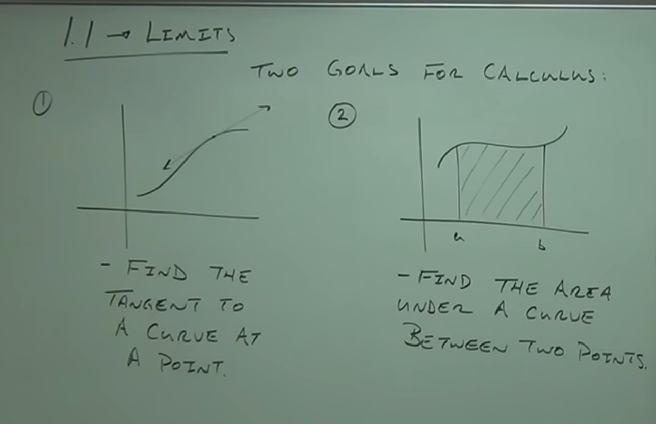
  • Objective 1: Find the tangent line to a curve (slope) at a given point.
  • Objective 2: Find the area under a curve between two points.

Ｔｈｅ Ｐｒｏｂｌｅｍ ｏｆ ｔｈｅ Ｔａｎｇｅｎｔ

• [5:56]. Introduction to the problem of the tangent: how to find the equation of the tangent line to a curve at a given point. – [📷image-1] – [📷image-2]
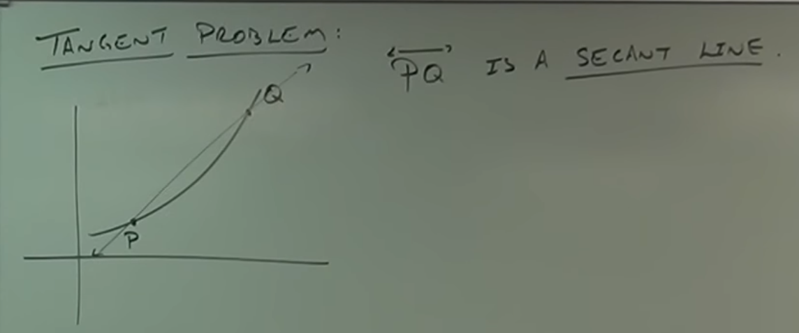
  • [7:24]. The concept of the secant line is introduced as an approximation to the tangent line.
    • 🕵 To find the tangent line to a curve at a point: First, we need to calculate the slope of the tangent line. But…
      • We can’t find the slope with just one point!
      • So we use another nearby point on the curve, called 𝑸.
    • 📌 The line through the given point 𝑷 and the nearby point 𝑸: 𝑷𝑸⃡, is called a secant line.
  • [08:28]. Is this secant line 𝑷𝑸⃡ a good approximation of the tangent line? How could we get a better approximation?
    • 𝑷 is a fixed point, but 𝑸 is a movable point.
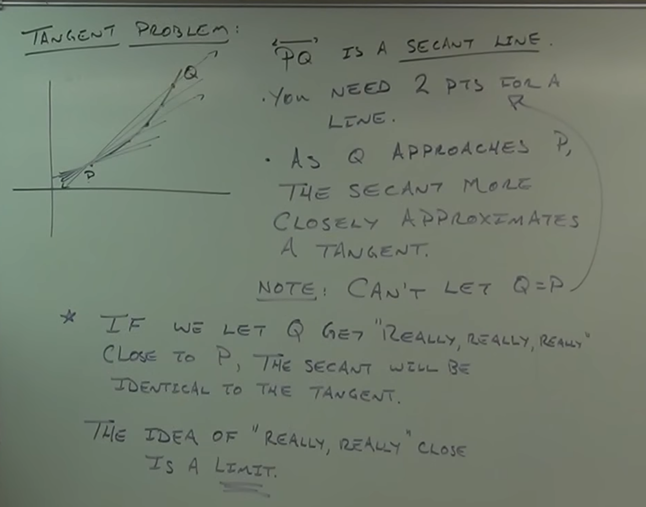
  • [9:40]. It is explained how to move 𝑸 on the secant line so that it approaches the tangent line.
    • If we move 𝑸 closer along the curve, the approximation becomes even better.
      • When can we stop? Can we get as close as possible to point 𝑷?
      • We can’t actually reach point 𝑷, because we need two points to define a line.
      • The idea is to move point 𝑸 so, so, so, so close to 𝑷 that the secant line becomes practically identical to the tangent line at point 𝑷.
  • [13:35]. The concept of a limit is introduced: bringing one point closer to another without them being the same.
    • 𝑰𝒏 𝒄𝒂𝒍𝒄𝒖𝒍𝒖𝒔, 𝙩𝙬𝙤 𝙥𝙤𝙞𝙣𝙩𝙨 𝙘𝙖𝙣 𝙗𝙚 𝙞𝙣𝙛𝙞𝙣𝙞𝙩𝙚𝙨𝙞𝙢𝙖𝙡𝙡𝙮 𝙘𝙡𝙤𝙨𝙚 𝙩𝙤 𝙚𝙖𝙘𝙝 𝙤𝙩𝙝𝙚𝙧 — 𝙣𝙤𝙩 𝙚𝙭𝙖𝙘𝙩𝙡𝙮 𝙩𝙝𝙚 𝙨𝙖𝙢𝙚, 𝙗𝙪𝙩 𝙨𝙤 𝙘𝙡𝙤𝙨𝙚 𝙩𝙝𝙖𝙩 𝙩𝙝𝙚 𝙙𝙞𝙛𝙛𝙚𝙧𝙚𝙣𝙘𝙚 𝙗𝙚𝙘𝙤𝙢𝙚𝙨 𝙣𝙚𝙜𝙡𝙞𝙜𝙞𝙗𝙡𝙚. 𝑻𝙝𝒊𝙨 𝙞𝙨 𝒕𝙝𝒆 𝒇𝙤𝙪𝙣𝒅𝙖𝒕𝙞𝒐𝙣 𝙤𝒇 𝒕𝙝𝒆 𝒄𝙤𝙣𝙘𝙚𝙥𝒕 𝒐𝒇 𝙡𝒊𝙢𝒊𝙩𝙨.
      • The name “infinitesimal calculus” comes from its core idea: working with quantities that are infinitesimally small — values that are not zero, but so close to zero that they behave almost like it. For example, when finding the tangent line to a curve at a point, we imagine a second point Q getting $\boxed{\textcolor{#FFD54F}{\textbf{infinitesimally close}}}$ to the fixed point 𝑷. As 𝑸 approaches 𝑷, the secant line 𝑷𝑸⃡ becomes almost indistinguishable from the tangent line. This process — letting the distance between two points shrink infinitely — is what makes calculus so powerful. It allows us to define limits, derivatives, and integrals.
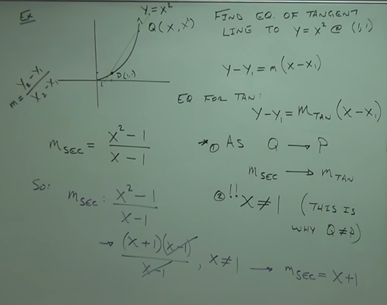
• [18:40]. 🧩 Example –: Find the equation of the tangent line to the curve $y=x^2$ at the point 𝑷(1, 1) – [📷image-1] – [📷image-2] – [📷image-3]
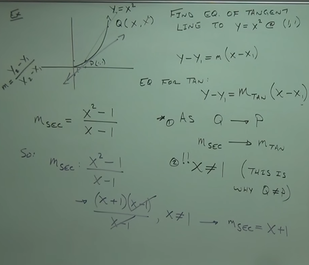
  • Define a moving point 𝑸 on the curve: 𝑸($x,x^2$).
  • Recall the slope formula for a line between two points:

    $m=\dfrac{y_2-y_1}{x_2-x_1}$

  • [23:30]. Compute the slope of the secant line between 𝑷 and 𝑸:

    $m_{\text{sec}}=\dfrac{x^2-1}{x-1}=\dfrac{(x+1)(x-1)}{x-1}=x+1$ (as long as $x\neq1$)

  • ⚠ Why $x\neq1$?
    • We can’t divide by zero.
    • This is why 𝑸 ≠ 𝑷. We use 𝑸 to approach 𝑷, not coincide.
  • 📌 IDEA: move point 𝑸 so, so, so, so close to 𝑷 that the secant line becomes practically identical to the tangent line at point 𝑷.
    • The slope of the secant line is related to the slope of the tangent line using the concept of a limit: As 𝑸 → 𝑷, $m_{\text{sec}} \to m_{\text{tan}}$
    • IDEA: What happens to the value of $m_{\text{sec}}$ as $x\to1$, that is, as 𝑸 → 𝑷?
      • Imagine 𝑸 getting nfinitesimally close to the fixed point 𝑷(1, 1)
        • if 𝑸(4,𝑦) we get $m_{\text{sec}}\big|_{x=4}=4+1=5$
        • if 𝑸(2,𝑦) we get $m_{\text{sec}}\big|_{x=2}=2+1=3$
        • if 𝑸(1.5,𝑦) we get $m_{\text{sec}}\big|_{x=1.5}=1.5+1=2.5$
        • . . .
        • if 𝑸(1.0000...1,𝑦) we get $m_{\text{sec}}\big|_{x=1.0000...1}=1.0000...1+1=2.0000...1$
        • Because $x$ is infinitely close to 1, we can now “jump” to 1 — the secant has effectively become the tangent.
          • $\boxed{\textcolor{#FFD54F}{\textbf{Infinitesimally close}}}$: We are visualizing the limit as a progressive approach where there is no practical difference between being infinitely close to the point and being at the point itself.
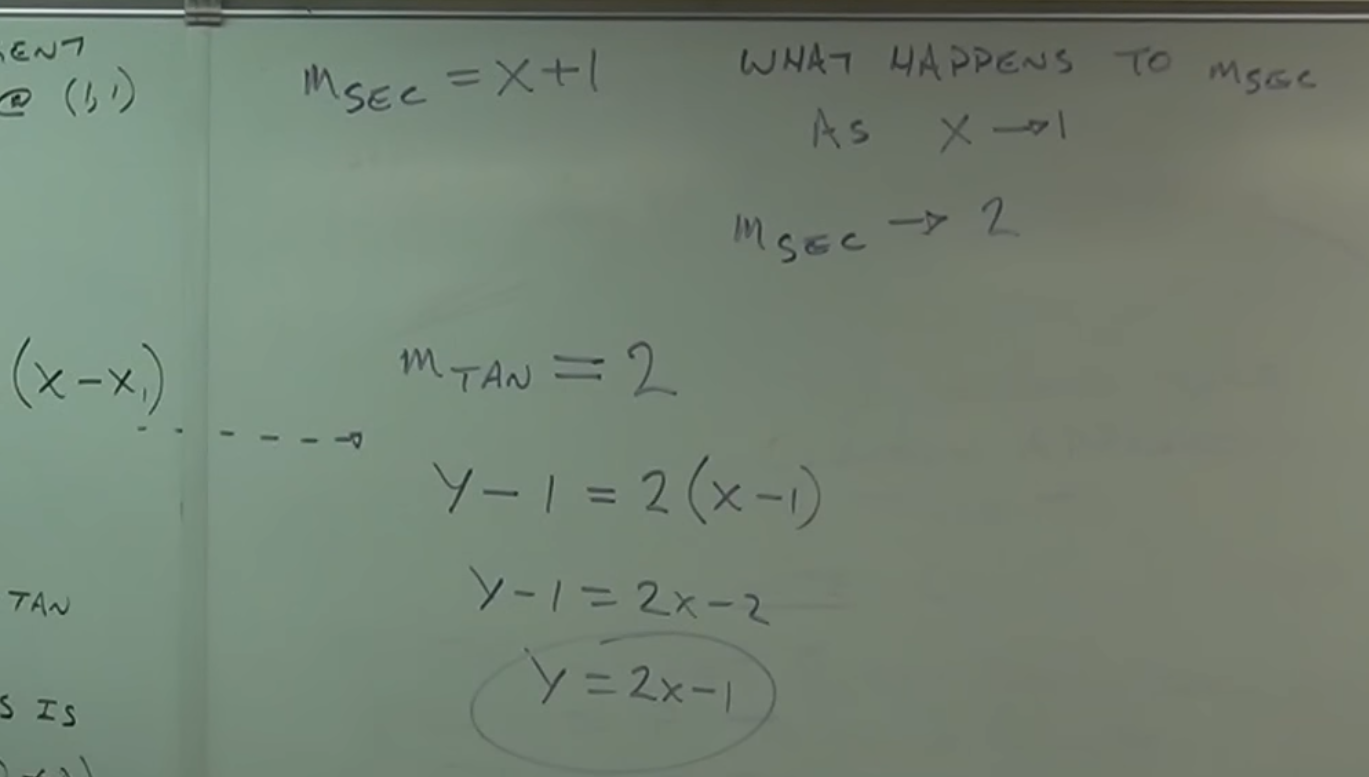
      • $m_{\text{sec}}\big|_{x=1}=1+1=2$ so as $x\to1$ $m_{\text{sec}} \to 2$
        • Hence, because $m_{\text{sec}} \to m_{\text{tan}}$, $m_{\text{tan}}=2$
  • Conclusion: the slope of the tangent line at 𝑷(1, 1) is 2.
  • Find the tangent line using point-slope form: $y-1=2(x-1)\;\Rightarrow\;y=2x-1$

Ｔｈｅ Ｐｒｏｂｌｅｍ ｏｆ ｔｈｅ Ａｒｅａ

• [36:40]. Brief introduction to the area problem – [📷image]
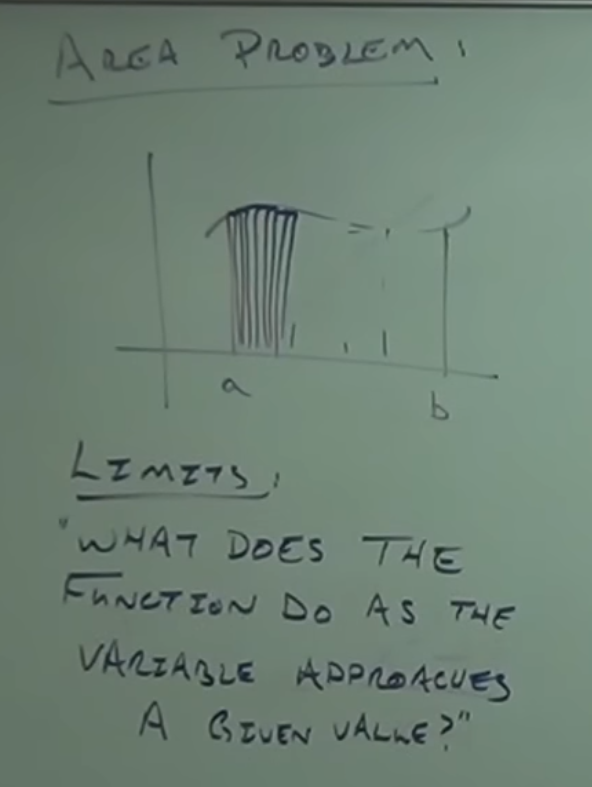
  • The question is posed: how to find the area under a curve.
  • The idea of approximating the area with rectangles is introduced.
  • It is explained that by using an infinite number of rectangles, the area is calculated exactly.

Ｄｅｆｉｎｉｔｉｏｎ ｏｆ ａ Ｌｉｍｉｔ

• [39:20]. The concept of a limit is defined in general terms:
  • What does the function do as a variable approaches a given value?
• [40:55]. 🧩 Example – : What does the function $f(x)=x^2$ do as $x$ approaches 2? – [📷image]
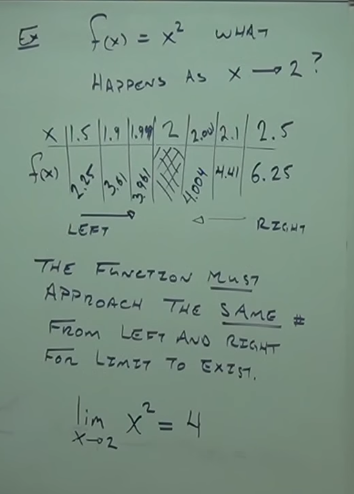
  • A table of values is constructed to approximate the limit.
  • It is observed that the function approaches 4 from both the right and the left.
• [44:40]. The formal notation of the limit is introduced:
  • 𝙏𝒉𝒆 𝒇𝙪𝙣𝙘𝒕𝙞𝙤𝙣 𝒎𝙪𝙨𝒕 𝙖𝙥𝙥𝙧𝙤𝙖𝙘𝙝 𝒕𝙝𝙚 𝙨𝙖𝙢𝙚 𝙫𝙖𝙡𝙪𝙚 𝒇𝙧𝙤𝙢 𝙡𝙚𝙛𝙩 𝒂𝙣𝙙 𝙧𝙞𝙜𝙝𝙩 𝒇𝙤𝙧 𝙡𝙞𝙢𝙞𝒕 𝙩𝙤 𝙚𝙭𝙞𝙨𝙩.
  • $\displaystyle \lim_{x\to a} f(x)=L;\;\; \displaystyle \lim_{x\to 2} x^2 = 4$
• It is emphasized that the limit does not depend on the value of the function at the point, but on its behavior near the point.
• [47:14]. 🧩 Example – What are limits?: $\displaystyle \lim_{x\to 1}\dfrac{x-1}{x^2-1}$ – [📷image]
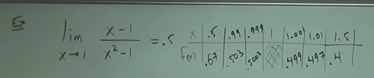
  • Since the function has a hole at $x=1$, it is best to create a table again.
  • $\displaystyle \lim_{x\to 1}\dfrac{x-1}{x^2-1}=0.5$

Ｏｎｅ－ｓｉｄｅｄ Ｌｉｍｉｔｓ

• [57:30]. Introduction to one-sided limits – [📷image]
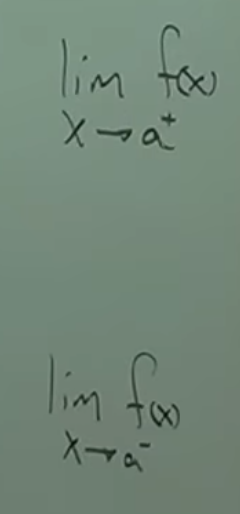
  • The notation for one-sided limits is explained.
    • right-hand limits $\displaystyle \lim_{x\to a^+} f(x)$
    • left-hand limits $\displaystyle \lim_{x\to a^-} f(x)$
• [1:00:00]. 🧩 Example –: Calculate the one-sided limits of a function represented graphically as $x$ approaches 2 – [📷image]
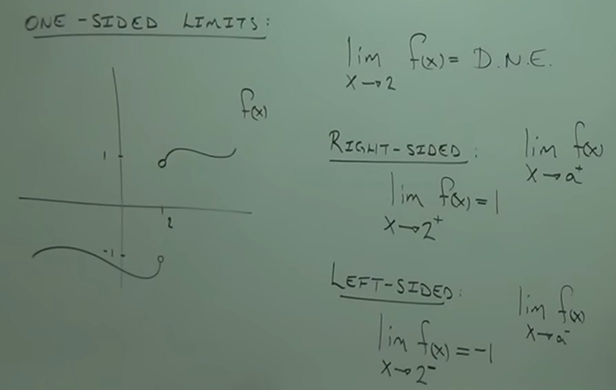
  • It is observed that $\displaystyle \lim_{x\to 2^+} f(x) = 1$ and $\displaystyle \lim_{x\to 2^-} f(x) = -1$.
  • [1:02:32]. 𝐍𝐎𝐓𝐄: 𝑻𝙝𝒆 𝒄𝙤𝙣𝙙𝒊𝙩𝒊𝙤𝙣 𝒇𝙤𝙧 𝒕𝒉𝒆 𝒆𝙭𝒊𝙨𝙩𝒆𝙣𝒄𝒆 𝒐𝒇 𝙖 𝙡𝒊𝙢𝒊𝒕 𝙞𝒔 𝒔𝙩𝒂𝒕𝒆𝒅:
    • 𝙏𝒉𝙚 𝙤𝒏𝙚-𝙨𝒊𝙙𝙚𝙙 𝙡𝒊𝙢𝒊𝙩𝒔 𝒎𝙪𝙨𝒕 𝙗𝒆 𝒆𝙦𝒖𝒂𝙡.
      • $\boxed{\displaystyle \lim_{x\to a^+} f(x) = \lim_{x\to a^-} f(x) \;\Longleftrightarrow\; \text{The limit exists}}$
  • It is concluded that $\displaystyle \lim_{x\to 2} f(x)$ does not exist: D.N.E.
• [1:06:00]. 🧩 Example –: Calculate $\displaystyle \lim_{x\to 2} g(x)$ – [📷image]
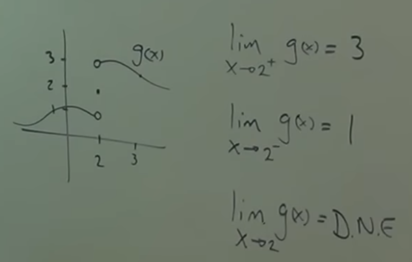
  • It is confirmed that $\displaystyle \lim_{x\to 2^+} g(x) = 3$ and $\displaystyle \lim_{x\to 2^-} g(x) = 1$.
  • It is concluded that $\displaystyle \lim_{x\to 2} g(x)$ D.N.E. because the one-sided limits are different.
• [1:10:20]. 🧩 Example –: Calculate $\displaystyle \lim_{x\to 5} h(x)$ – [📷image]
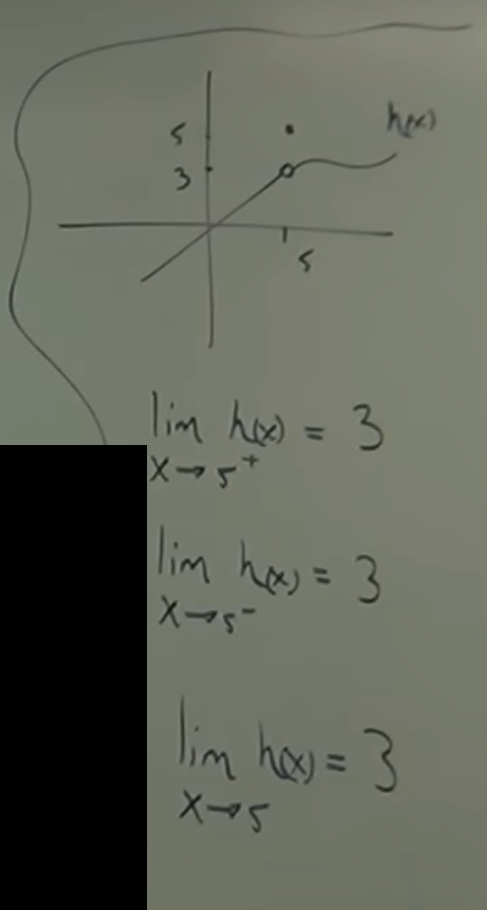
  • It is confirmed that $\displaystyle \lim_{x\to 5^+} h(x) = 3$ and $\displaystyle \lim_{x\to 5^-} h(x) = 3$.
  • It is concluded that $\displaystyle \lim_{x\to 5} h(x)$ exists and is equal to 3 because the one-sided limits are equal.

Ｉｎｆｉｎｉｔｅ Ｌｉｍｉｔｓ ａｎｄ Ａｓｙｍｐｔｏｔｅｓ

• [1:14:12]. 🧩 Example –: Find limit of $f(x)=\dfrac{1}{x}$ as $x \to 0$ – [📷image]
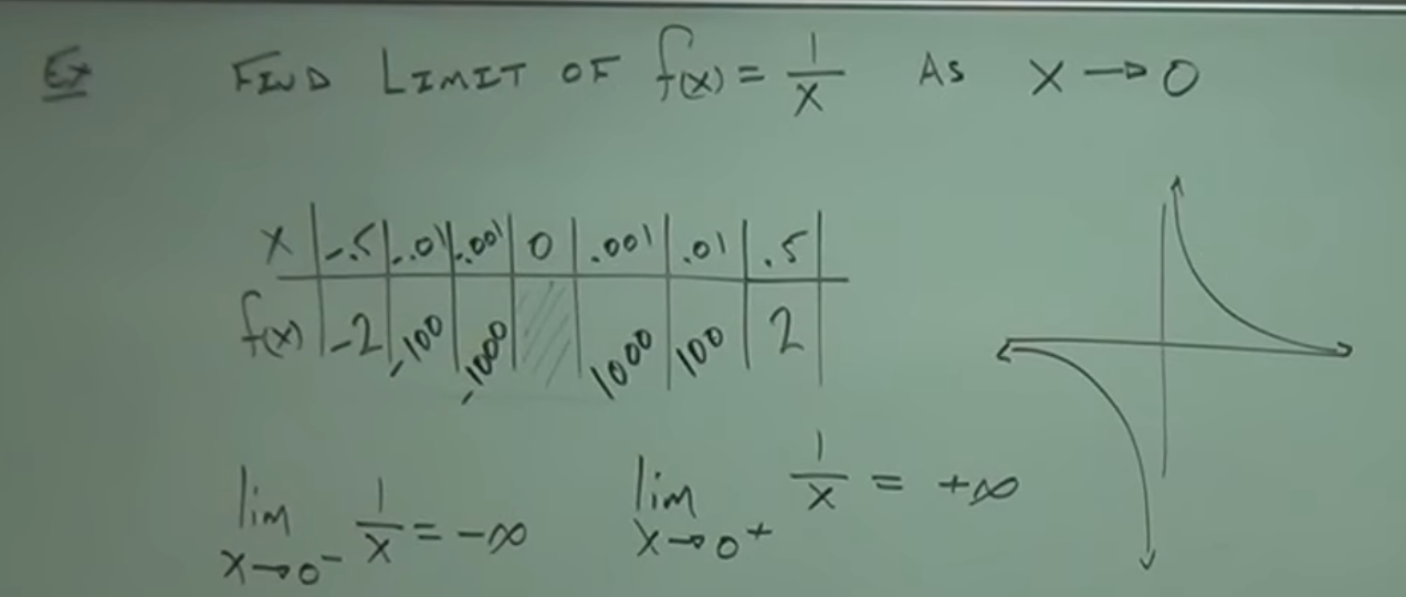
  • What happens to the function $\dfrac{1}{x}$ as $x$ approaches $0$.
  • A table of values is constructed to approximate the one-sided limits.
  • [1:17:43]. It is observed that $\displaystyle \lim_{x\to 0^-}\dfrac{1}{x}=-\infty$ and $\displaystyle \lim_{x\to 0^+}\dfrac{1}{x}=+\infty$.
• [1:19:43]. The infinite limit is related to the existence of a vertical asymptote. – [📷image]
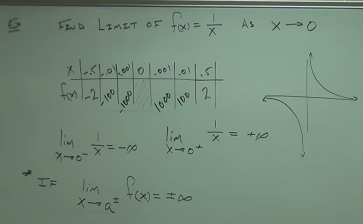
  • $\boxed{\displaystyle \lim_{x\to a^\pm} f(x) = \pm\infty \;\;\Longleftrightarrow\;\;\text{vertical asymptote}}$ .
• [1:22:15]. The four possible cases of vertical asymptotes and their relation to infinite limits are graphically explained. – [📷image]
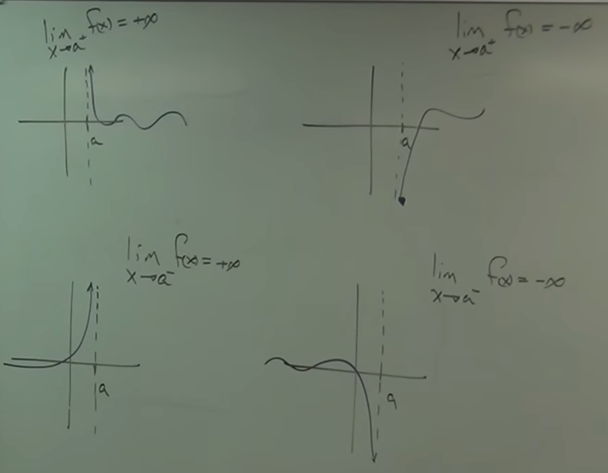
  • The behavior of the function in each case is analyzed.
  • The limit exists only when both one-sided limits tend to the same infinite value: – [📷image]
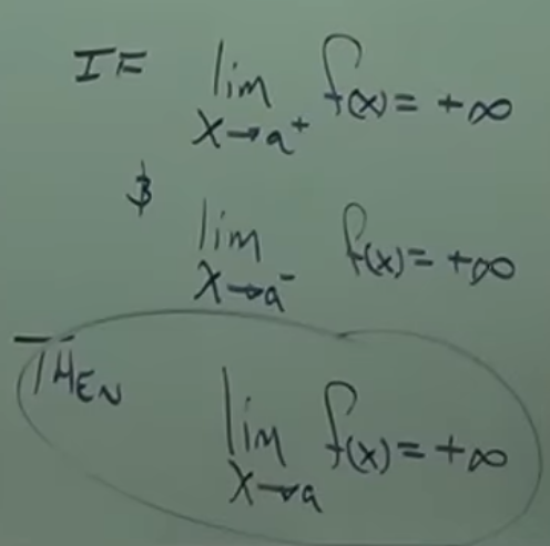
    • $\displaystyle \lim_{x\to a^+} f(x) = +\infty$ and $\displaystyle \lim_{x\to a^-} f(x) = +\infty$ ⟶ vertical asymptote at $x=a$
    • $\displaystyle \lim_{x\to a^+} f(x) = -\infty$ and $\displaystyle \lim_{x\to a^-} f(x) = -\infty$ ⟶ vertical asymptote at $x=a$
    • $\displaystyle \lim_{x\to a^+} f(x) = +\infty$ and $\displaystyle \lim_{x\to a^-} f(x) = -\infty$ ⟶ opposite-sided divergence (no single limit)
    • $\displaystyle \lim_{x\to a^+} f(x) = -\infty$ and $\displaystyle \lim_{x\to a^-} f(x) = +\infty$ ⟶ opposite-sided divergence (no single limit)
  • In the first two cases, the infinite limit “exists” (in the extended sense) and defines the vertical asymptote.
  • In the last two cases, the function still has a vertical asymptote at $x=a$, but the two sides diverge in opposite directions, so the limit does not exist.