Ｃａｌｃｕｌｕｓ　１　ｌｅｃｔｕｒｅ　１．４：　Cｏｎｔｉｎｕｉｔｙ　Oｆ　Fｕｎｃｔｉｏｎｓ

Ｃｏｎｔｉｎｕｉｔｙ

• 0:11. 𝐈𝐧𝐭𝐮𝐢𝐭𝐢𝐯𝐞 𝐃𝐞𝐟𝐢𝐧𝐢𝐭𝐢𝐨𝐧 𝐨𝐟 𝐂𝐨𝐧𝐭𝐢𝐧𝐮𝐢𝐭𝐲 – [📷image]
  • A function is continuous if it can be drawn without lifting the pencil from the paper.
    • It has no holes, jumps, or asymptotes.
• 1:45. 𝐌𝐚𝐭𝐡𝐞𝐦𝐚𝐭𝐢𝐜𝐚𝐥 𝐃𝐞𝐟𝐢𝐧𝐢𝐭𝐢𝐨𝐧 𝐨𝐟 𝐂𝐨𝐧𝐭𝐢𝐧𝐮𝐢𝐭𝐲 – [📷image]
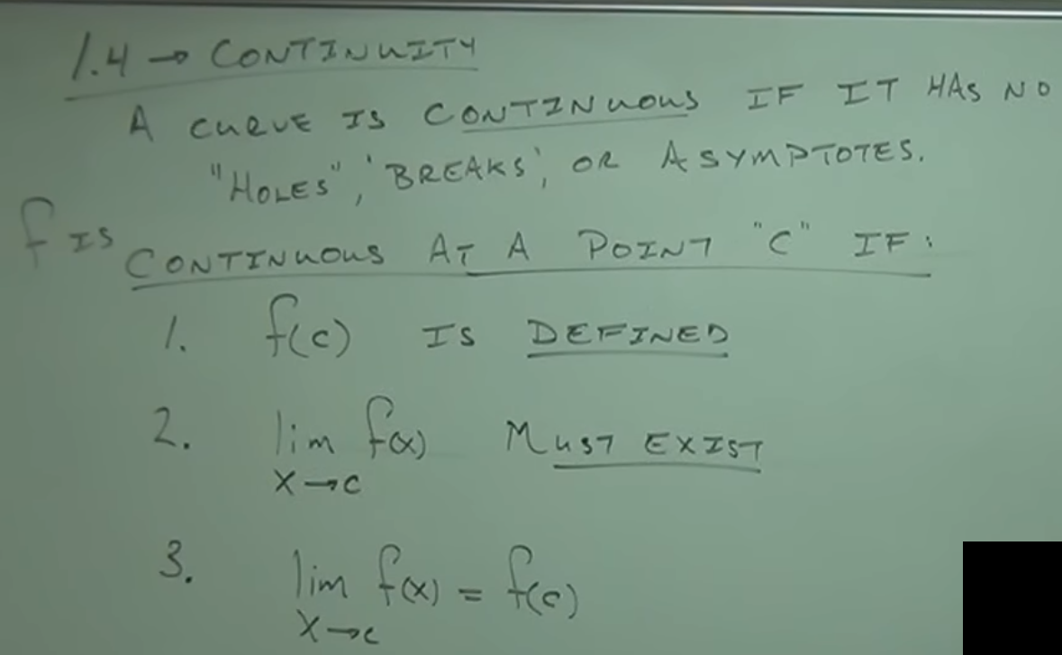
  • A function is continuous at a point 𝒄 if it meets three conditions:
    • (ⅰ). The function is defined at that point.
      $𝒇(𝒄)$ is defined.
    • (ⅱ). $\displaystyle \lim_{𝒙\to 𝒄} 𝒇(𝒙)$ the limit of the function as 𝒙 approaches 𝒄 exists. Meaning the function approaches the same value from both sides.
    • (ⅲ). The value of the function at point 𝒄 is equal to the limit of the function as 𝒙 approaches 𝒄.
      $\displaystyle \lim_{𝒙\to 𝒄} 𝒇(𝒙)=𝒇(𝒄)$
  • Important distinction:
    • Necessary conditions → What must happen for continuity.
    • Sufficient conditions → What guarantees continuity.
  • Necessary and Sufficient: Continuity at a point 𝒙 = 𝒄 requires all three conditions:
    • Condition (ⅰ): $𝒇(𝒄)$ is defined → Necessary.
    • Condition (ⅱ): $\displaystyle \lim_{𝒙\to 𝒄} 𝒇(𝒙)$ exists → Necessary.
    • Condition (ⅲ): $\displaystyle \lim_{𝒙\to 𝒄} 𝒇(𝒙)=𝒇(𝒄)$ → Sufficient (if this holds and the previous two, the function is continuous).
• 4:41. 𝐂𝐨𝐧𝐭𝐢𝐧𝐮𝐢𝐭𝐲 𝐢𝐧 𝐓𝐞𝐫𝐦𝐬 𝐨𝐟 𝐃𝐫𝐚𝐰𝐢𝐧𝐠 𝐚 𝐅𝐮𝐧𝐜𝐭𝐢𝐨𝐧
  • If you trace a continuous function, you reach a point, fill in the point, and continue without interruptions.
• 5:35. 𝐆𝐫𝐚𝐩𝐡𝐢𝐜𝐚𝐥 𝐄𝐱𝐚𝐦𝐩𝐥𝐞𝐬 𝐨𝐟 𝐂𝐨𝐧𝐭𝐢𝐧𝐮𝐢𝐭𝐲 𝐚𝐧𝐝 𝐃𝐢𝐬𝐜𝐨𝐧𝐭𝐢𝐧𝐮𝐢𝐭𝐲
  • Removable Discontinuity
    • Case A: A Graph with a Hole at 𝒙 = 𝐜 and $𝒇(𝐜)$ not exists – [📷image]
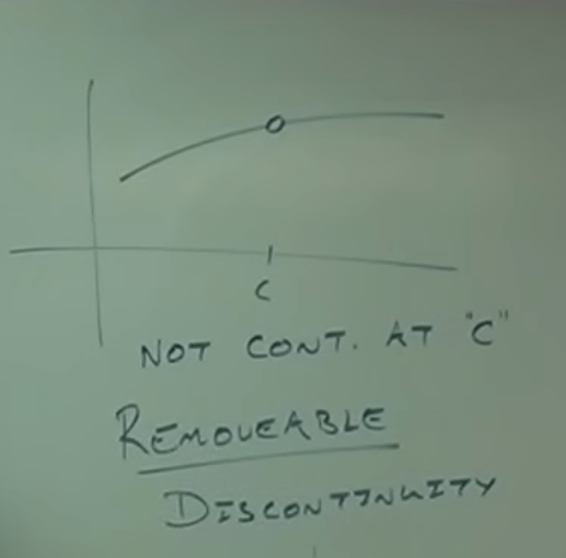
      • The function is not defined at 𝒙 = 𝐜, which directly breaks continuity at that point.
      • The limit exists as 𝒙 approaches 𝐜, but it is not equal to the function value (which is undefined).
      • This is a 𝒓𝒆𝒎𝒐𝒗𝒂𝒃𝒍𝒆 𝒅𝒊𝒔𝒄𝒐𝒏𝒕𝒊𝒏𝒖𝒊𝒕𝒚, since the "hole" could be filled by defining the function at 𝒙 = 𝐜.
    • Case B 10:48. : A Graph with a Hole at 𝒙 = 𝐜 and $𝒇(𝐜)$ exists – [📷image]
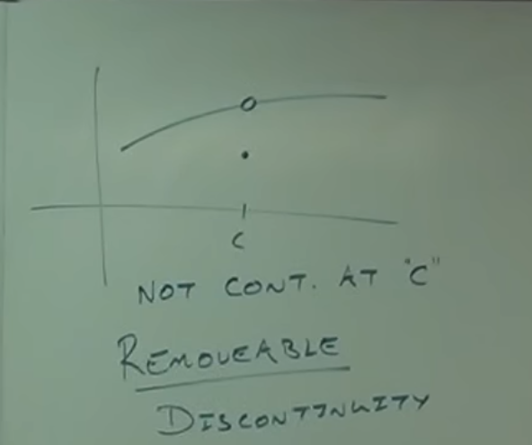
      • The function is defined at 𝒙 = 𝒄, but it is not equal to the limit.
      • The limit exists as 𝒙 approaches 𝐜, but differs from the function value.
      • This is still a 𝒓𝒆𝒎𝒐𝒗𝒂𝒃𝒍𝒆 𝒅𝒊𝒔𝒄𝒐𝒏𝒕𝒊𝒏𝒖𝒊𝒕𝒚, since we could redefine $𝒇(𝐜)$ to match the limit and make the function continuous.
  • 7:30. Jump Discontinuity – [📷image]
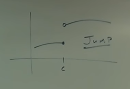
    • A Graph with a Jump at 𝒙 = 𝒄
      • The function is defined at 𝒙 = 𝒄.
      • The limit does not exist at 𝒙 = 𝒄 because the function approaches different values from the left and right.
      • This is a 𝙟𝒖𝙢𝒑 𝒅𝙞𝙨𝙘𝙤𝙣𝙩𝙞𝙣𝙪𝙞𝙩𝙮.
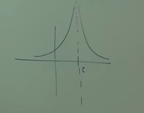
  • 9:20. Infinite Discontinuity – [📷image-1] – [📷image-2]
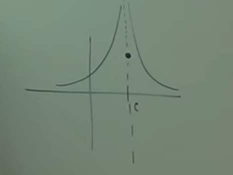
    • A Graph with a Vertical Asymptote at 𝒙 = 𝒄
      • The function is (image-2) or not (image-1) defined at 𝒙 = 𝒄.
      • The limit exists at 𝒙 = 𝒄 and is infinite.
      • This is an 𝙞𝙣𝙛𝙞𝙣𝙞𝙩𝙚 𝙙𝙞𝙨𝙘𝙤𝙣𝙩𝙞𝙣𝙪𝙞𝙩𝙮.--
  • 11:09. Summary of Types of Discontinuity
    • There are three main types of discontinuity:
      • 1. Infinite discontinuity (associated with vertical asymptotes).
      • 2. Jump discontinuity.
      • 3. Removable discontinuity (a "hole" in the graph).
    • A removable discontinuity can be "filled in" by defining the function at that point.
    • Rational functions typically show removable discontinuities or vertical asymptotes.
    • Jump discontinuities usually appear in piecewise-defined functions.
  • 13:07. 🧩 Examples, Are these continuous at x = 2?
    • $𝒇(𝒙)=\dfrac{𝒙^{2}-4}{𝒙-2}$ – [📷image]
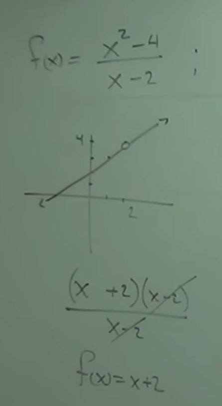
      • Domain check:
        • $𝒙=2$ makes the denominator zero ⇒ the original formula is undefined at $𝒙=2$
      • Algebraic simplification (for $𝒙\neq 2$):
        • $𝒙^{2}-4=(𝒙-2)(𝒙+2)$
        • Then $𝒇(𝒙)=\dfrac{(𝒙-2)(𝒙+2)}{𝒙-2}=𝒙+2$ (valid only when $𝒙\neq 2$)
      • Limit at $𝒙=2$: ▣ $\displaystyle \lim_{𝒙\to 2} 𝒇(𝒙)=\lim_{𝒙\to 2}(𝒙+2)=4$
      • Continuity test at $𝒙=2$:
        • Need: (i) $𝒇(2)$ exists, (ii) $\displaystyle \lim_{𝒙\to 2} 𝒇(𝒙)$ exists, (iii) they are equal.
        • Here, $𝒇(2)$ does not exist (undefined by the original expression), although the limit is $4$.
        • ⇒ 𝒇 is NOT continuous at $𝒙=2$. (Removable discontinuity: a “hole” at $(2,4)$.)
    
    
    • 16:20. 𝓰(𝒙) is defined as: $\displaystyle𝓰(𝒙)=\begin{cases}\dfrac{𝒙^{2}-4}{𝒙-2}, & \text{if } 𝒙\neq 2 \\[6pt]3, & \text{if } 𝒙=2\end{cases}$ – [📷image]
      
      
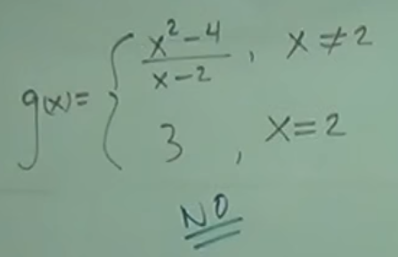
      • Condition (ⅰ): $𝒇(2)$ is defined → Necessary✅
      • Condition (ⅱ): $\displaystyle \lim_{𝒙\to 2} 𝒇(𝒙)$ exists → Necessary✅
      • Condition (ⅲ): $\displaystyle \lim_{𝒙\to 2} 𝒇(𝒙)\neq 𝒇(2)$ → Sufficient ❌
    
    
    • 17:36. 𝒉(𝒙) = $\displaystyle\begin{cases}\dfrac{𝒙^{2}-4}{𝒙-2}, & \text{if } 𝒙\neq 2 \\[6pt]4, & \text{if } 𝒙=2\end{cases} $ – [📷image]
      
      
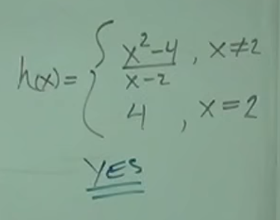
      • Condition (ⅰ): $𝒇(2)$ is defined → Necessary✅
      • Condition (ⅱ): $\displaystyle \lim_{𝒙\to 2} 𝒇(𝒙)$ exists → Necessary✅
      • Condition (ⅲ): $\displaystyle \lim_{𝒙\to 2} 𝒇(𝒙)=𝒇(2)$ → Sufficient ✅
• 18:25. 𝐂𝐨𝐧𝐭𝐢𝐧𝐮𝐢𝐭𝐲 𝐨𝐧 𝐚𝐧 𝐈𝐧𝐭𝐞𝐫𝐯𝐚𝐥 – [📷image]
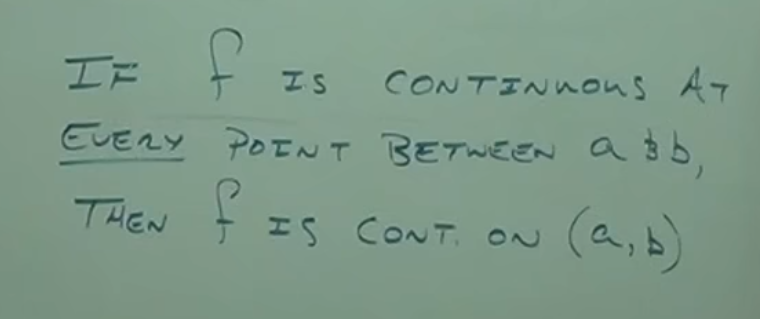
  • If a function is continuous at e͟v͟e͟r͟y͟ point between a and b, it is said to be continuous on the open interval $(a,b)$.
• 19:35. 𝐂𝐨𝐧𝐭𝐢𝐧𝐮𝐢𝐭𝐲 𝐚𝐭 𝐭𝐡𝐞 𝐄𝐧𝐝𝐩𝐨𝐢𝐧𝐭𝐬 𝐨𝐟 𝐚𝐧 𝐈𝐧𝐭𝐞𝐫𝐯𝐚𝐥
  • 🧩 Example – Introduction: Continuity at endpoints of an interval – [📷image]
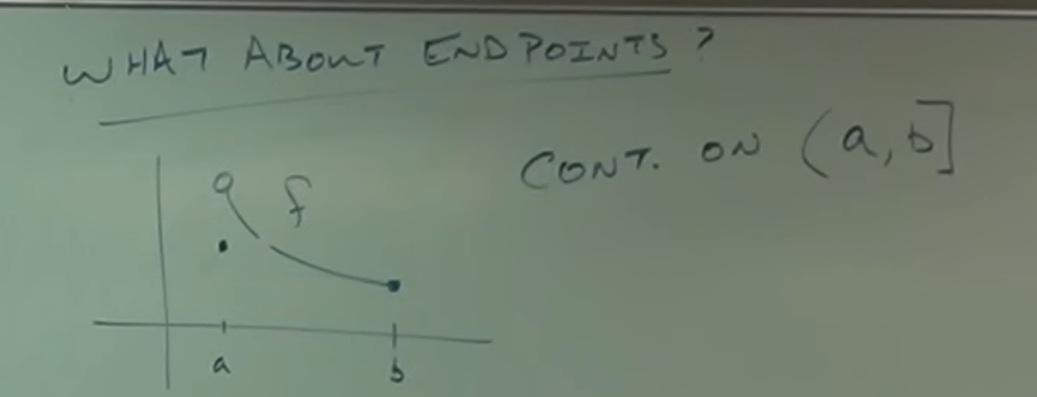
  • To determine if a function is continuous on a closed interval $[a,b]$:
    • ❶ You must verify continuity on the open interval $(a,b)$
    • ❷ You must verify continuity at the endpoints $a$ and $b$.
  • At the endpoints of an interval, one-sided limits are used to verify continuity.
  • For a function to be continuous at an endpoint, the one-sided limit must exist and be equal to the value of the function at that endpoint.
    • 22:50. 𝐌𝐚𝐭𝐡𝐞𝐦𝐚𝐭𝐢𝐜𝐚𝐥 𝐃𝐞𝐟𝐢𝐧𝐢𝐭𝐢𝐨𝐧 𝐨𝐟 𝐎𝐧𝐞-𝐒𝐢𝐝𝐞𝐝 𝐂𝐨𝐧𝐭𝐢𝐧𝐮𝐢𝐭𝐲 – [📷image]
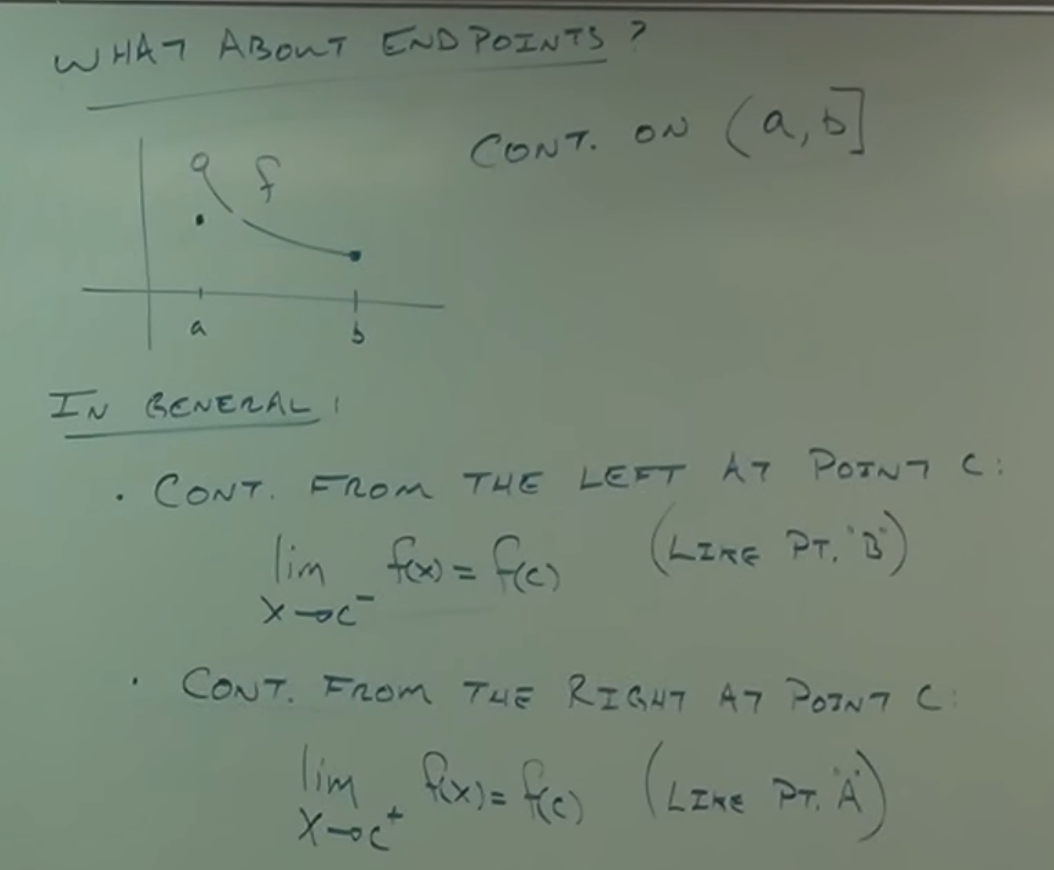
      • Continuity from the left: The limit of $𝒇(𝒙)$ as 𝒙 approaches $c$ from the left must equal $𝒇(𝒄)$.
        • $\displaystyle \lim_{𝒙\to 𝒄^-} 𝒇(𝒙)=𝒇(𝒄)$
      • Continuity from the right: The limit of $f(𝒙)$ as 𝒙 approaches $c$ from the right must equal $f(𝒄)$.
        • $\displaystyle \lim_{𝒙\to 𝒄^+} 𝒇(𝒙)=𝒇(𝒄)$
  • 25:41. 🧩 Example – : $𝒇(𝒙)=\sqrt{16-𝒙^{2}}$ on the Closed Interval $[-4,4]$ – [📷image]
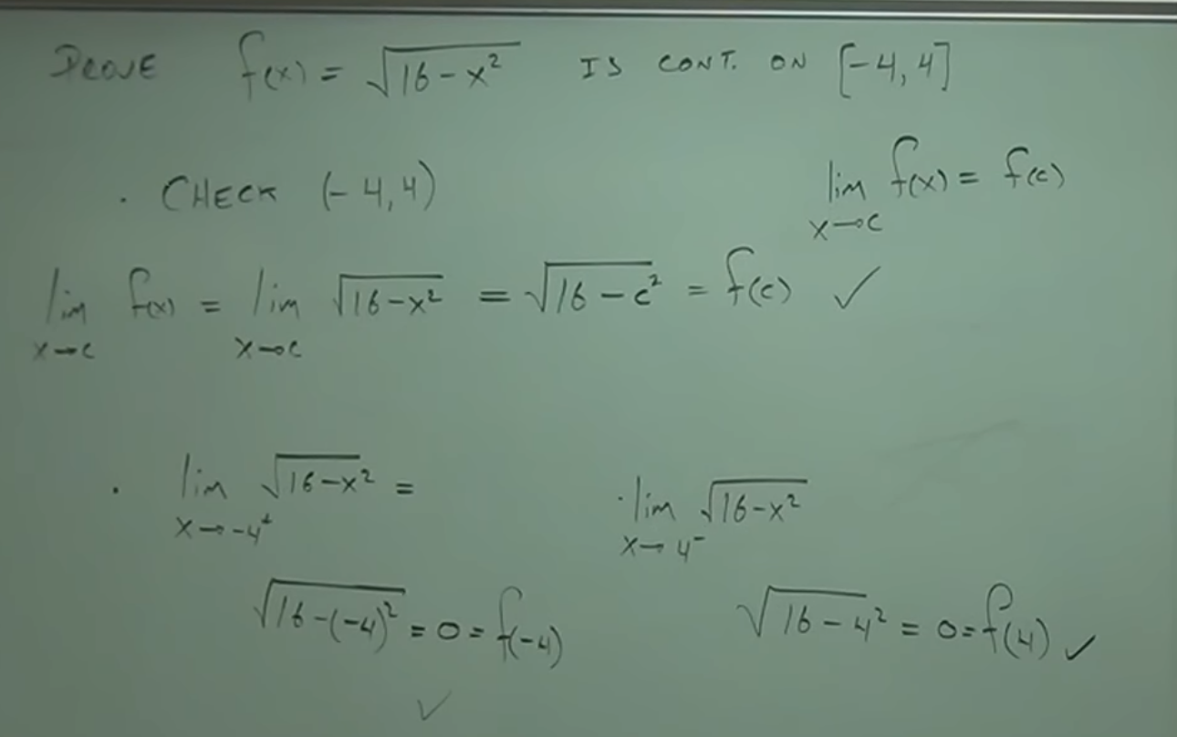
    • Steps for the Demonstration:
      • ❶ Verify continuity on the open interval $(-4,4)$.
      • ❷ Verify continuity from the left at $-4$ and verify continuity from the right at $4$.
      • 29:11. ❶ Demonstration of Continuity on the Open Interval $(-4,4)$
        • To show that the function is continuous at $𝒙=𝒄$, we verify that: $\displaystyle \lim_{𝒙\to 𝒄} 𝒇(𝒙)=𝒇(𝒄)$
        • The expression $\sqrt{16-𝒙^{2}}$ is defined for values of 𝒙 such that $16-𝒙^{2}\ge 0$ → $𝒙\in[-4,4]$
        • $\displaystyle \lim_{𝒙\to 𝒄} 𝒇(𝒙)=\lim_{𝒙\to 𝒄}\sqrt{16-𝒙^{2}}=\sqrt{16-𝒄^{2}}=𝒇(𝒄)\;$ ✓
        • It must be shown that the limit of $𝒇(𝒙)$ as 𝒙 approaches $c$ is equal to $f(𝒄)$ for any value of $𝒄$ between $-4$ and $4$.
          • $\displaystyle \lim_{𝒙\to 𝒄} 𝒇(𝒙)=𝒇(𝒄)$ $𝒙\in[-4,4]$
      • 32:46. ❷ Demonstration of One-Sided Continuity at the Endpoints ($𝒄=-4$ and $𝒄=4$)
        • Continuity from the left: The limit of $𝒇(𝒙)$ as 𝒙 approaches $𝒄$ from the left must equal $f(𝒄)$.
          • Since there are no points to the right of $4$ within the interval, we only consider the left-hand limit.
          • $\displaystyle \lim_{𝒙\to 𝒄^-} 𝒇(𝒙)=𝒇(𝒄)\;\to\; \lim_{𝒙\to 4^-}\sqrt{16-(4)^{2}}=0=𝒇(4)=𝒇(𝒄)$
        • Continuity from the right: The limit of $f(𝒙)$ as 𝒙 approaches $c$ from the right must equal $f(𝒄)$.
          • Similarly, Since there are no points to the left of $-4$ within the interval, we only consider the right-hand limit.
          • $\displaystyle \lim_{𝒙\to 𝒄^+} 𝒇(𝒙)=𝒇(𝒄)\;\to\; \lim_{𝒙\to -4^+}\sqrt{16-(-4)^{2}}=0=𝒇(-4)=𝒇(𝒄)$
      • 📝 N͟O͟T͟E͟:
        • 𝐎𝐧𝐞-𝐒𝐢𝐝𝐞𝐝 𝐂𝐨𝐧𝐭𝐢𝐧𝐮𝐢𝐭𝐲: 𝐁𝐚𝐬𝐢𝐜 𝐂𝐨𝐧𝐜𝐞𝐩𝐭𝐬
          • One-sided continuity refers to the existence of a limit from either the left or the right that matches the value of the function at a specific point. The general definition is:
            • Continuity from the left:
              • $\displaystyle \lim_{𝒙\to 𝒄^-} 𝒇(𝒙)=𝒇(𝒄)$
            • Continuity from the right:
              • $\displaystyle \lim_{𝒙\to 𝒄^+} 𝒇(𝒙)=𝒇(𝒄)$
        • 𝐀𝐩𝐩𝐥𝐢𝐜𝐚𝐭𝐢𝐨𝐧 𝐢𝐧 𝐂𝐥𝐨𝐬𝐞𝐝 𝐈𝐧𝐭𝐞𝐫𝐯𝐚𝐥𝐬
          • In a closed interval such as $[-4,4]$, the endpoints ($𝒙=-4$ and $𝒙=4$) 𝒉𝒂𝒗𝒆 𝒐𝒏𝒍𝒚 𝒐𝒏𝒆 𝒔𝒊𝒅𝒆 𝒘𝒊𝒕𝒉𝒊𝒏 𝒕𝒉𝒆 𝒅𝒐𝒎𝒂𝒊𝒏. Therefore:
            • At $𝒙=-4$, we check 𝒐𝒏𝒍𝒚 right-hand continuity $[-4\leftarrow\ldots,4]$
            • At $𝒙=4$, we check 𝒐𝒏𝒍𝒚 left-hand continuity $[-4,\ldots\to 4]$
          • This is because the function is not defined beyond those endpoints, so it makes no sense to evaluate the limit from both sides.
      • 34:53. Conclusion of the Demonstration
        • It has been shown that the function is continuous on the open interval and at the endpoints.
        • Therefore, the function is continuous on the closed interval $[-4,4]$.
• 35:50. 𝐏𝐫𝐨𝐩𝐞𝐫𝐭𝐢𝐞𝐬 𝐨𝐟 𝐂𝐨𝐧𝐭𝐢𝐧𝐮𝐢𝐭𝐲 𝐢𝐧 𝐎𝐩𝐞𝐫𝐚𝐭𝐢𝐨𝐧𝐬 𝐰𝐢𝐭𝐡 𝐅𝐮𝐧𝐜𝐭𝐢𝐨𝐧𝐬 – [📷image]
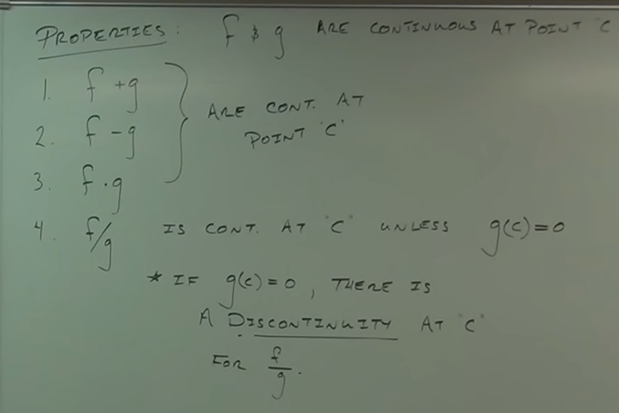
  • If 𝒇 and 𝓰 are continuous at a point 𝒄, then:
    • $𝒇+𝓰$ is continuous at 𝒄.
    • $𝒇-𝓰$ is continuous at 𝒄.
    • $𝒇\cdot 𝓰$ is continuous at 𝒄.
  • $\dfrac{𝒇}{𝓰}$ is continuous at 𝒄 unless $𝓰(𝒄)=0$.
    • 38:20. Discontinuities in Rational Functions
      • If $𝓰(𝒄)=0$ in a rational function $\dfrac{𝒇}{𝓰}$, then there is a discontinuity at 𝒄.
        • The discontinuity can be a hole or an asymptote.
• 40:50. 𝐂𝐨𝐧𝐭𝐢𝐧𝐮𝐢𝐭𝐲 𝐨𝐟 𝐏𝐨𝐥𝐲𝐧𝐨𝐦𝐢𝐚𝐥𝐬 – [📷image]
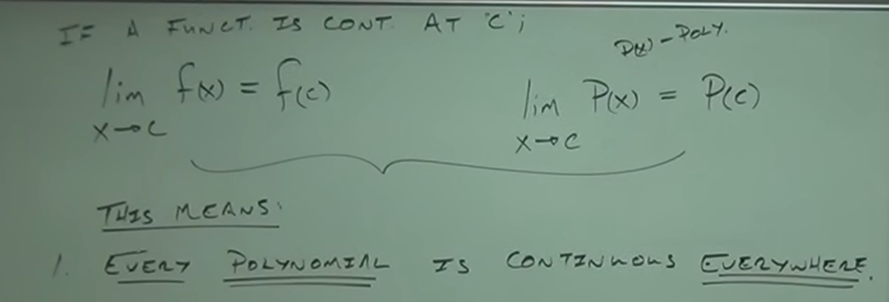
  • ⑴ Recall (ⅲ):
    • $\displaystyle \lim_{𝒙\to 𝒄} 𝒇(𝒙)=𝒇(𝒄)$ ⇔ 𝒇 is continuous at 𝒄
  • ⑵ Recall the property of polynomial limits: the limit of a polynomial as 𝒙 approaches any point can be evaluated simply by substituting 𝒙 with that point.
    • $ \forall 𝒄\in\mathbb{R}:\; \displaystyle \lim_{𝒙\to 𝒄} P(𝒙)=P(𝒄)$
  • ⑴ and ⑵ implies that all polynomials are continuous at all points.
    • $ \forall 𝒄\in\mathbb{R}:\; \displaystyle \lim_{𝒙\to 𝒄} P(𝒙)=P(𝒄)\;\; \Leftrightarrow\;\; P$ is continuous at every point in $\mathbb{R}$
• 44:10. 𝐂𝐨𝐧𝐭𝐢𝐧𝐮𝐢𝐭𝐲 𝐨𝐟 𝐑𝐚𝐭𝐢𝐨𝐧𝐚𝐥 𝐅𝐮𝐧𝐜𝐭𝐢𝐨𝐧𝐬 $\dfrac{𝐏(𝒙)}{𝐐(𝒙)}$ – [📷image]
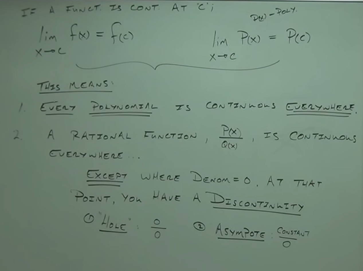
  • Combining the continuity property of polynomials with the continuity property of function division, it is concluded that every rational function is continuous at all points except where the denominator $Q(𝒙)$ is zero. At that point you have a Discontinuity.
    • 47:15. 𝑯͟𝒐͟𝒍͟𝒆͟𝒔͟ ͟𝒂͟𝒏͟𝒅͟ ͟𝑨͟𝒔͟𝒚͟𝒎͟𝒑͟𝒕͟𝒐͟𝒕͟𝒆͟𝒔͟ ͟𝒊͟𝒏͟ ͟𝑹͟𝒂͟𝒕͟𝒊͟𝒐͟𝒏͟𝒂͟𝒍͟ ͟𝑭͟𝒖͟𝒏͟𝒄͟𝒕͟𝒊͟𝒐͟𝒏͟𝒔͟ ͟𝒂͟𝒔͟ ͟𝑫͟𝒊͟𝒔͟𝒄͟𝒐͟𝒏͟𝒕͟𝒊͟𝒏͟𝒖͟𝒊͟𝒕͟𝒊͟𝒆͟𝐬͟.͟
      • Hole $(0/0)$: In a rational function, if a common factor can be canceled by factoring the numerator and the denominator, the discontinuity corresponding to that factor is a hole.
      • Asymptote $(\text{constant}/0)$: If a factor of the denominator cannot be canceled, the discontinuity corresponding to that factor is an asymptote.
  • 50:07. 🧩 Example – How to Find Discontinuities in a Rational Function: $𝒇(𝒙)=\dfrac{𝒙^{2}-4}{𝒙^{2}+𝒙-6}$ – [📷image]
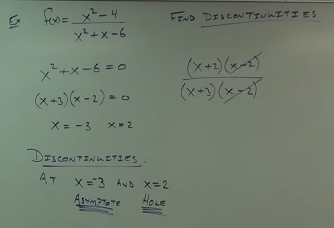
    • Procedure: Discontinuities are found by setting the denominator to zero and solving the equation.
      • Discontinuities: $𝒙=2$ and $𝒙=-3$.
      • Factor the function: $𝒇(𝒙)=\dfrac{(𝒙+2)(𝒙-2)}{(𝒙+3)(𝒙-2)}$
      • It is observed that the factor $(𝒙-2)$ cancels out $(0/0)$, indicating a 𝐡𝐨𝐥𝐞 at $𝒙=2$.
      • The factor $(𝒙+3)$ does not cancel out $(\text{constant}/0)$, indicating an asymptote at $𝒙=3$.
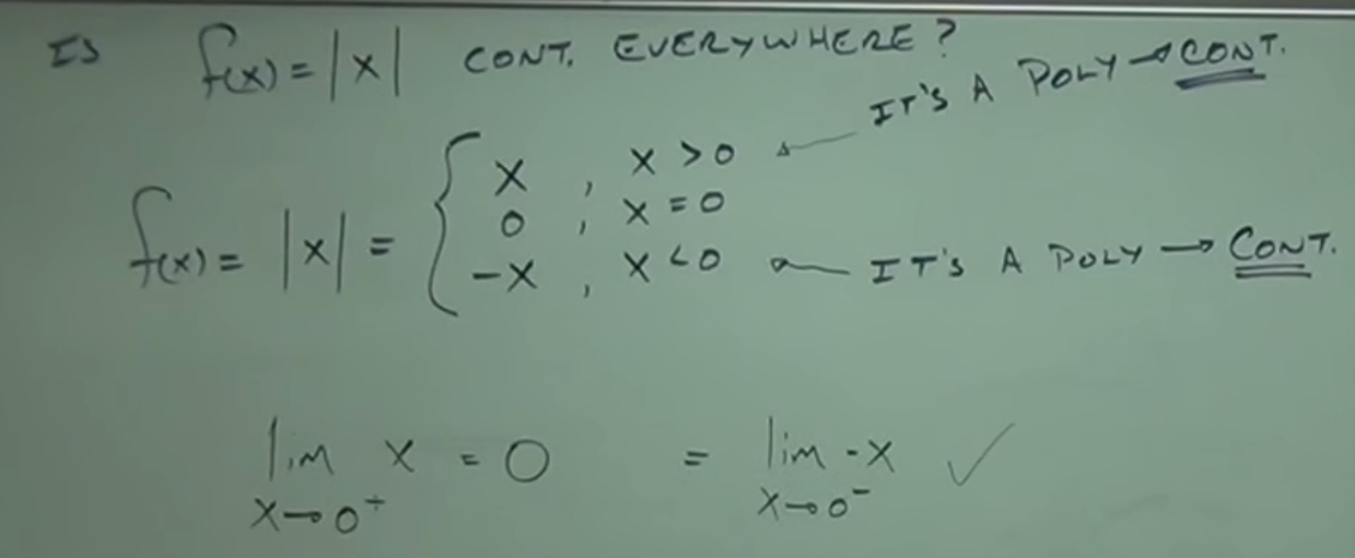
• 55:00. 𝐃𝐞𝐦𝐨𝐧𝐬𝐭𝐫𝐚𝐭𝐢𝐨𝐧 𝐨𝐟 𝐂𝐨𝐧𝐭𝐢𝐧𝐮𝐢𝐭𝐲 𝐨𝐟 𝐭𝐡𝐞 𝐀𝐛𝐬𝐨𝐥𝐮𝐭𝐞 𝐕𝐚𝐥𝐮𝐞 𝐅𝐮𝐧𝐜𝐭𝐢𝐨𝐧 – [📷image]
  
  
  • $𝒇(𝒙)=|𝒙|=$ $\displaystyle\begin{cases}𝒙, & \text{if } 𝒙>0 \quad \text{→ it's a polynomial → continuous} \\[6pt]0, & \text{if } 𝒙=0 \\6pt]-𝒙, & \text{if } 𝒙<0 \quad \text{→ it's a polynomial → continuous}\end{cases}$
  
  
  • Procedure: The function is defined piecewise to avoid issues with limits at the endpoints.
  • Continuity on Open Intervals:
    • For $𝒙>0$, the function is simply $𝒇(𝒙)=𝒙$, which is a polynomial and therefore continuous.
    • For $𝒙<0$, the function is $𝒇(𝒙)=-𝒙$, which is also a polynomial and therefore continuous.
  • Continuity at $𝒙=0$:
    • The important thing here is to verify the definition of continuity at $𝒙=0$; $\displaystyle \lim_{𝒙\to 0}|𝒙|=0$
    • Continuity from the left: $\displaystyle \lim_{𝒙\to 0^-}|𝒙|=\lim_{𝒙\to 0^-}(-𝒙)=0$
    • Continuity from the right: $\displaystyle \lim_{𝒙\to 0^+}|𝒙|=\lim_{𝒙\to 0^+}𝒙=0$
• 1:00:30. 𝐂𝐨𝐧𝐭𝐢𝐧𝐮𝐢𝐭𝐲 𝐨𝐟 𝐂𝐨𝐦𝐩𝐨𝐬𝐢𝐭𝐞 𝐅𝐮𝐧𝐜𝐭𝐢𝐨𝐧𝐬 – [📷image]
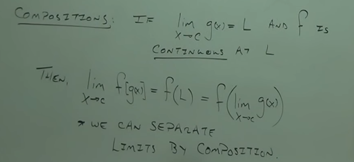
  • 1:00:52. T̳ʜ̳ᴇ̳ᴏ̳ʀ̳ᴇ̳ᴍ̳ 1:
    • I̲f̲ the limit of $𝓰(𝒙)$ as 𝒙 approaches 𝒄 exists and is equal to $L$, and $𝒇$ is continuous at $L$,
      • t̲h̲e̲n̲ the limit of $𝒇(𝓰(𝒙))$ as 𝒙 approaches 𝒄 is equal to $𝒇(L)$.
    • Conditions:
      • $𝓰$ must have a limit at $𝒄$ (does NOT need to be continuous at $𝒄$).
      • $𝒇$ must be continuous at $L$ (the limit value of $𝓰(𝒙)$).
    • Usage:
      • This theorem is used to compute limits of composite functions.
    • 1:02:17. Demonstration:
      • The definition of the limit is used to express the limit of $𝓰(𝒙)$ as 𝒙 approaches 𝒄 as $L$.
      • The continuity of $𝒇$ at $L$ is used to express $𝒇(L)$ as the limit of $𝒇(𝒙)$ as 𝒙 approaches $L$.
        • This follows from the definition of continuity:
          • I̲f̲ a function $𝒇$ is continuous at a point $L$,
            • t̲h̲e̲n̲ $\displaystyle \lim_{𝒙\to L} 𝒇(𝒙)=𝒇(L)$
        • This identity allows us to replace $L$ in $𝒇(L)$ with a limit in the next step of the proof.
      • $L$ is substituted with the limit of $𝓰(𝒙)$ as 𝒙 approaches $𝒄$ in the expression for $𝒇(L)$.
        • $\displaystyle \lim_{𝒙\to 𝒄} 𝒇(𝓰(𝒙))=𝒇(L)=𝒇\!\big(\lim_{𝒙\to 𝒄} 𝓰(𝒙)\big)$
      • 1:04:27. Conclusion: The limit of a composite function can be evaluated by taking the limit of the inner function and then applying the outer function, provided the outer function is continuous at that value:
        • I̲f̲ $\displaystyle \lim_{𝒙\to 𝒄} 𝓰(𝒙)=L$ and $𝒇$ is continuous at $L$,
          • t̲h̲e̲n̲ $\displaystyle \lim_{𝒙\to 𝒄} 𝒇(𝓰(𝒙))=𝒇\!\big(\lim_{𝒙\to 𝒄} 𝓰(𝒙)\big)=𝒇(L)$.
  • 1:04:56. 🧩 Example – How to Use Continuity of Composite Functions: $\displaystyle \lim_{𝒙\to 4} 𝒇(𝒙)=\lvert 10-3𝒙^{2}\rvert$ – [📷image]
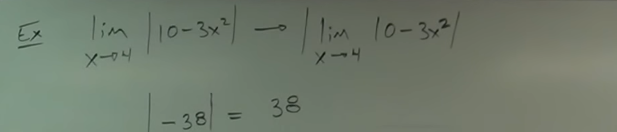
    • Procedure:
      • It is observed that the function is the composition of $𝓰(𝒙)=10-3𝒙^{2}$ and the absolute value function $𝒇(𝒙)=|𝒙|$.
      • Since both the inner function $𝓰(𝒙)=10-3𝒙^{2}$ (a polynomial) and the outer function $𝒇(𝒙)=|𝒙|$ are continuous at the relevant points, the theorem on continuity of composite functions can be applied.
    • 1:07:01. Calculation of the Limit:
      • The limit of $𝓰(𝒙)$ as 𝒙 approaches $4$ is calculated: $\displaystyle \lim_{𝒙\to 4}(10-3𝒙^{2})=-38$.
      • The absolute value function is applied to the result: $\big\lvert \lim_{𝒙\to 4}(10-3𝒙^{2}) \big\rvert=38$.
      • Conclusion: $\displaystyle \lim_{𝒙\to 4}\lvert 10-3𝒙^{2}\rvert=38$.
  • 1:07:50.T̳ʜ̳ᴇ̳ᴏ̳ʀ̳ᴇ̳ᴍ̳ 2: – [📷image]
    • I̲f̲ $𝒇: Y\to Z$ and $𝓰: X\to Y$ are functions continuous at all points,
      • t̲h̲e̲n̲ the composition $𝒇\circ 𝓰: X\to Z$ defined by $(𝒇\circ 𝓰)(𝒙)=𝒇(𝓰(𝒙))$ is also continuous at all points.
    • Conditions:
      • $𝓰$ must be continuous at all points in its domain.
      • $𝒇$ must be continuous on the image of $𝓰$ (i.e., at every $𝓰(𝒙)$).
    • Usage:
      • Used to prove that the composition $𝒇(𝓰(𝒙))$ is continuous.
  • 🔍 Key Difference:
    • The first theorem focuses on limits and requires $𝒇$ to be continuous only at one point ($L$).
    • The second theorem is about continuity and requires both functions to be continuous on their respective domains, so that their composition is also continuous.
• 1:08:49. 𝐂𝐨𝐧𝐭𝐢𝐧𝐮𝐢𝐭𝐲 𝐨𝐟 𝐈𝐧𝐯𝐞𝐫𝐬𝐞 𝐅𝐮𝐧𝐜𝐭𝐢𝐨𝐧𝐬 – [📷image]
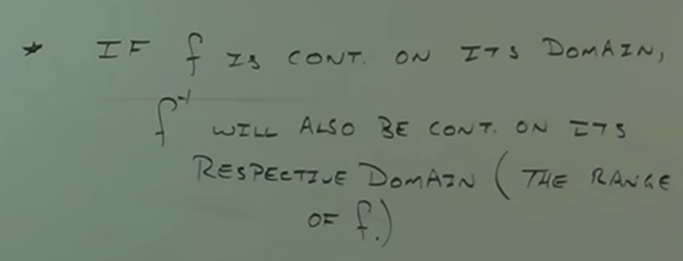
  • T̳ʜ̳ᴇ̳ᴏ̳ʀ̳ᴇ̳ᴍ̳:
    • I̲f̲ $𝒇$ is continuous on its domain,
      • t̲h̲e̲n̲ $𝒇^{-1}$ is continuous on its domain, which is equal to the range of $𝒇$.
  • 1:10:40. 🧩 Example – Continuity of an Inverse Function: $𝒇(𝒙)=𝒙^{3}$ – [📷image]
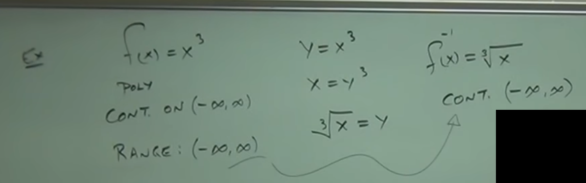
    • Continuity of $𝒇$: Since $𝒇$ is a polynomial, it is continuous on its entire domain, which is the set of all real numbers.
    • Range of $𝒇$: The range of $𝒇$ is also the set of all real numbers.
    • Inverse Function: $𝒇^{-1}(𝒙)=\sqrt[3]{𝒙}$.
    • Continuity of $𝒇^{-1}$: According to the theorem on continuity of inverse functions, $𝒇^{-1}$ is continuous on its domain, which is equal to the range of $𝒇$, that is, the set of all real numbers.

Ｉｎｔｅｒｍｅｄｉａｔｅ Ｖａｌｕｅ Ｔｈｅｏｒｅｍ

• 1:12:21. 𝐈𝐧𝐭𝐞𝐫𝐦𝐞𝐝𝐢𝐚𝐭𝐞 𝐕𝐚𝐥𝐮𝐞 𝐓𝐡𝐞𝐨𝐫𝐞𝐦 – [📷image]
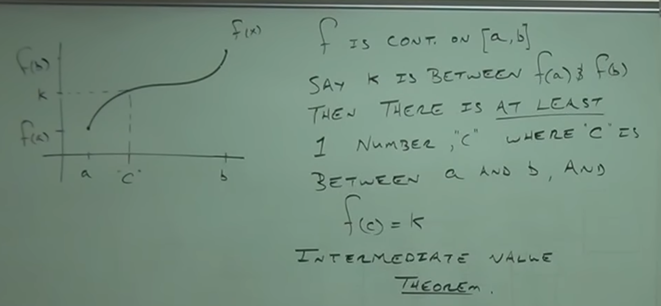
  • Introduction: The Intermediate Value Theorem is presented as an 𝒂𝒑𝒑𝒍𝒊𝒄𝒂𝒕𝒊𝒐𝒏 𝒐𝒇 𝒄𝒐𝒏𝒕𝒊𝒏𝒖𝒊𝒕𝒚.
  • General Idea: If a function is continuous on a closed interval, and a value lies between the function values at the endpoints, then there is at least one point in the interval where the function takes that value.
    • If a function is continuous on a closed interval $[\mathfrak{a},𝒃]$, and the values at the endpoints are $𝒇(\mathfrak{a})=5$ and $𝒇(𝒃)=9$, then for any number between $5$ and $9$ (for example, $6$), there is at least one number $𝒄$ in the interval $(\mathfrak{a},𝒃)$ such that: $f(𝒄)=6$
    • The key idea is continuity: a continuous function cannot “skip” values. It must pass through every value between $𝒇(\mathfrak{a})$ and $𝒇(𝒃)$.
  • 1:15:43. Formal Statement:
    • T̳ʜ̳ᴇ̳ᴏ̳ʀ̳ᴇ̳ᴍ̳:
      • I̲f̲ $𝒇$ is continuous on the closed interval $[\mathfrak{a},𝒃]$, and $k$ is a value between $𝒇(\mathfrak{a})$ and $𝒇(𝒃)$,
        • t̲h̲e̲n̲ there exists at least one number $𝒄$ in the interval $(\mathfrak{a},𝒃)$ such that $𝒇(𝒄)=k$
• 1:17:35. 𝐈𝐧𝐭𝐞𝐫𝐩𝐫𝐞𝐭𝐚𝐭𝐢𝐨𝐧 𝐨𝐟 𝐭𝐡𝐞 𝐈𝐧𝐭𝐞𝐫𝐦𝐞𝐝𝐢𝐚𝐭𝐞 𝐕𝐚𝐥𝐮𝐞 𝐓𝐡𝐞𝐨𝐫𝐞𝐦
  • If a function is continuous on an interval, it cannot _skip_ or _jump over_ any value between $𝒇(\mathfrak{a})$ and $𝒇(𝒃)$.
• 1:19:13. 𝐀𝐩𝐩𝐥𝐢𝐜𝐚𝐭𝐢𝐨𝐧 𝐨𝐟 𝐭𝐡𝐞 𝐈𝐧𝐭𝐞𝐫𝐦𝐞𝐝𝐢𝐚𝐭𝐞 𝐕𝐚𝐥𝐮𝐞 𝐓𝐡𝐞𝐨𝐫𝐞𝐦: 𝐀𝐩𝐩𝐫𝐨𝐱𝐢𝐦𝐚𝐭𝐢𝐧𝐠 𝐑𝐨𝐨𝐭𝐬 – [📷image]
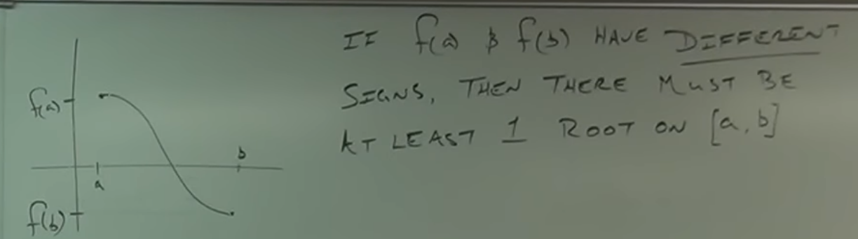
  • Introduction: The Intermediate Value Theorem can be used to approximate the roots of a function, that is, the points where the function crosses the 𝒙-axis.
  • Procedure:
    • An interval $[\mathfrak{a},𝒃]$ is sought where the function changes sign, that is, where $𝒇(\mathfrak{a})$ and $𝒇(𝒃)$ have opposite signs.
    • According to the Intermediate Value Theorem, if the function is continuous on $[\mathfrak{a},𝒃]$ and $𝒇(\mathfrak{a})$ and $𝒇(𝒃)$ have 𝐨𝐩𝐩𝐨𝐬𝐢𝐭𝐞 𝐬𝐢𝐠𝐧𝐬, then there is at least one root $𝒄$ in the interval $(\mathfrak{a},𝒃)$, that is $𝒇(𝒄)=0$.
    • Here $k=0$
• 1:23:25. 🧩 Example – 𝐇𝐨𝐰 𝐭𝐨 𝐀𝐩𝐩𝐫𝐨𝐱𝐢𝐦𝐚𝐭𝐞 𝐑𝐨𝐨𝐭𝐬 𝐔𝐬𝐢𝐧𝐠 𝐭𝐡𝐞 𝐈𝐧𝐭𝐞𝐫𝐦𝐞𝐝𝐢𝐚𝐭𝐞 𝐕𝐚𝐥𝐮𝐞 𝐓𝐡𝐞𝐨𝐫𝐞𝐦: – [📷image]
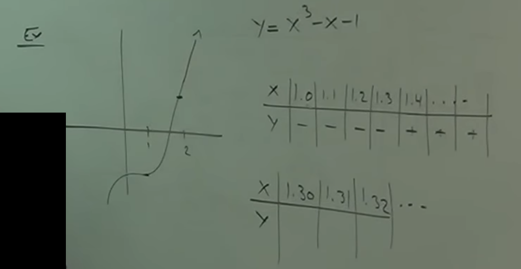
  • $𝒇(𝒙)=𝒙^{3}-𝒙-1$
  • Procedure:
    • An interval $[1,2]$ is found where the function changes sign. In this e𝒙ample, the interval is used.
    • A table is created with 𝒙-values in the interval and the function is evaluated at each 𝒙-value.
    • It is observed where the function changes sign. In this example, the sign change occurs between $𝒙=1.3$ and $𝒙=1.4$
    • The process is repeated with a smaller interval, in this case $[1.3,1.4]$, to obtain a more precise approximation of the root.
  • The process can be repeated with increasingly smaller intervals to obtain an approximation of the root as precise as desired.