Ｃａｌｃｕｌｕｓ　１　ｌｅｃｔｕｒｅ　３．６

　Hｏｗ　Tｏ　Sｋｅｔｃｈ　Gｒａｐｈｓ　Oｆ　Fｕｎｃｔｉｏｎｓ

Ｒｅｖｉｅｗ　ａｎｄ　ｉｎｉｔｉａｌ　ｅｘａｍｐｌｅ

• [0:17]. Curve sketching uses:
  • 𝒙-intercept and 𝑦-intercept.
  • Relative maxima and minima (extrema).
  • Concavity.
• Objective: Understand the shape of graphs without a graphing calculator, using calculus.

Ｓｔｅｐｓ　ｆｏｒ　ｃｕｒｖｅ　ｓｋｅｔｃｈｉｎｇ

• [0:41]. Steps for curvong sketchong [image]
• Presentation of the 🧩 Example –: $𝒇(𝒙)=(𝒙+2)(𝒙-1)^{2}$
• [1:18]. Step 1: Find the intercepts
  • Find 𝒙-intercepts:
    • Set 𝑦 = 0 and solve for 𝒙 (find the roots of the equation).
      • Simplify only if the equation is "easy": quadratic or lower degree, or if it is already factored.
    • $(𝒙+2)(𝒙-1)^{2}=0 \Rightarrow 𝒙+2=0 \;\to\; 𝒙=-2;\; 𝒙-1=0 \;\to\; 𝒙=1$
    • So the x-intercepts are: $𝒙=-2$ and $𝒙=1$.
  • Find the 𝑦-intercept:
    • Set 𝒙 = 0 and solve for 𝑦: $𝒇(0)=(0+2)(0-1)^{2}=2\cdot 1=2$
    • So the y-intercept is: $𝒚=2$.
• [6:04]. Step 2: Find asymptotes (only for rational $𝒇(𝒙)$)
  • Rational $𝒇(𝒙)$ can have vertical, horizontal asymptotes, and holes.
  • ❶ ᴠ̳ᴇ̳ʀ̳ᴛ̳ɪ̳ᴄ̳ᴀ̳ʟ̳ ̳ᴀ̳ꜱ̳ʏ̳ᴍ̳ᴘ̳ᴛ̳ᴏ̳ᴛ̳ᴇ̳ꜱ̳: Arise when the function tends to $±\infty$ as 𝒙 approaches a specific value.
    • Definition:
      • This occurs when:
        • (i) The function is undefined at $𝒙=𝒂$ because the d̳e̳n̳o̳m̳i̳n̳a̳t̳o̳r̳ ̳i̳s̳ ̳z̳e̳r̳o̳.
        • (ii) The factor causing the zero does not cancel with a factor in the numerator, meaning the discontinuity is non-removable and creates infinite behavior.
      • A vertical asymptote (VA) exists at $𝒙=𝒂$ if:
        • $\displaystyle \lim_{x\to a^-} 𝒇(𝒙)=\pm\infty$ or $\displaystyle \lim_{x\to a^+} 𝒇(𝒙)=\pm\infty$
        • (i.e., the function "blows up" on at least one side of $𝒙=𝒂$).
    • One-Sided Limits:
      • Rational functions or others with denominators approaching $0$ at $x=a$ often exhibit this behavior.
      • The function may diverge differently from each side:
        • 🧩 Example: $𝒇(𝒙)=\dfrac{1}{𝒙-a}$
          • $\displaystyle \lim_{x\to a^-} 𝒇(𝒙)=-\infty$, $\displaystyle \lim_{x\to a^+} 𝒇(𝒙)=+\infty$
          • $\displaystyle \lim_{x\to a} 𝒇(𝒙)$ D.N.E. (does not exist), but the vertical asymptote is still at $x=a$.
    • 🗒️ NOTE: The existence of a vertical asymptote does not require the two-sided limit to diverge in the same way or to exist at all. What matters is that at least one of the one-sided limits diverges to $±\infty$.
  • ❷ ʜ̳ᴏ̳ʟ̳ᴇ̳ꜱ̳ (Removable Discontinuities): Occur where the denominator equals zero, but the corresponding factor can be canceled.
    • Definition:
      • A hole occurs at $x=a$ if:
        • (i) The original function is undefined at $x=a$ due to a zero in the denominator.
        • (ii) That factor cancels with the numerator, allowing simplification.
        • (iii) The simplified expression is defined around $x=a$, but not at $x=a$ itself.
    • One-Sided Limits:
      • Check if both one-sided limits exist and match.Example:
        • $𝓰(𝒙)=\dfrac{(𝒙-1)(𝒙+1)}{(𝒙-1)(𝒙-2)}$ → Simplifies to: $𝓰(𝒙)=\dfrac{𝒙+1}{𝒙-2}$, for $𝒙\ne 1$.
      • In this case, $x=1$ is a hole:
        • The original form is undefined at $x=1$ (division by zero).
        • The simplified form is valid near $x=1$.
        • Evaluate: $\displaystyle \lim_{x\to 1^-} 𝓰(𝒙)$ and $\displaystyle \lim_{x\to 1^+} 𝓰(𝒙)$
          • If they are equal, the two-sided limit exists.
          • However, the function remains undefined at $x=1$, so there is a removable discontinuity.
    • 🗒️ NOTE:
      • A hole does not cause the function to diverge to $\infty$ like a vertical asymptote.
      • Instead, it’s a “missing point” on an otherwise continuous curve, where the limit exists but the function is undefined.
  • ❸ ʜ̳ᴏ̳ʀ̳ɪ̳ᴢ̳ᴏ̳ɴ̳ᴛ̳ᴀ̳ʟ̳ ̳ᴀ̳ꜱ̳ʏ̳ᴍ̳ᴘ̳ᴛ̳ᴏ̳ᴛ̳ᴇ̳ꜱ̳: Determined by evaluating the limit of a function as $𝒙\to \pm\infty$.
    • Definition:
      • A horizontal asymptote (HA) occurs when:
        • (i) $\displaystyle \lim_{x\to +\infty} 𝒇(𝒙)=\ell$ or $\displaystyle \lim_{x\to -\infty} 𝒇(𝒙)=\ell$ where $\ell$ is a real number.
        • (ii) The value $\ell$ represents the end behavior of the function — the value that $𝒇(𝒙)$ gets closer to as $𝒙$ becomes very large (positive or negative).
      • Unlike vertical asymptotes, which occur at specific finite values of $𝒙$, horizontal asymptotes describe how the function behaves as $𝒙$ tends toward infinity or negative infinity.
    • Directional (End) Behavior:
      • Evaluate the limits separately as $𝒙 \to +\infty$ and as $𝒙 \to -\infty$:
        • $\displaystyle \lim_{x\to +\infty} 𝒇(𝒙)$
        • $\displaystyle \lim_{x\to -\infty} 𝒇(𝒙)$
      • These are sometimes referred to as "one-sided" limits at infinity.
        • While not the same as limits from the left/right at a point (like $\displaystyle \lim_{x\to c^+}$ or $\displaystyle \lim_{x\to c^-}$), they illustrate how a function might tend to different horizontal asymptotes at each end of the 𝒙-axis.
    • 🗒️ NOTE:
      • Including examples of behavior as $𝒙 \to +\infty$ and $𝒙 \to -\infty$ helps students understand the concept of asymptotic behavior more clearly.
      • It reinforces that limits at infinity don’t always match:
        • A function may level off to one value as $𝒙 \to +\infty$, and a different one (or none) as $𝒙 \to -\infty$.
      • Just like with finite limits, the concept of a two-sided limit ($\displaystyle \lim_{x\to c} 𝒇(𝒙)$) only exists if both sides agree:
        • $\displaystyle \lim_{x\to c^-} 𝒇(𝒙)=\lim_{x\to c^+} 𝒇(𝒙)$
    • Summary:
      • If $\displaystyle \lim_{x\to \pm\infty} 𝒇(𝒙)=\ell$, then $y=\ell$ is a horizontal asymptote.
      • If the limits are different on each side, the function has two distinct horizontal asymptotes.
      • If no finite limit exists, then there is no horizontal asymptote in that direction.
• [9:07]. Step 3: Perform the first derivative test
  • The first derivative test provides critical numbers and intervals of increase/decrease.
  • The first derivative represents the rate of change of the function, or in simpler terms, how the function's value is increasing or decreasing.
  • Find the values of 𝒙 that make the numerator of $𝒇′(𝒙)$ equal to zero.
    • These are the critical points, candidates for maxima, minima, or points where the slope is zero (horizontal).
  • Find the values of 𝒙 that make the denominator of $𝒇′(𝒙)$ equal to zero:
    • These indicate places where the first derivative is undefined (possible vertical discontinuities or asymptotes).
  • It allows determining where maxima and minima are located and how the graph rises or falls.
• [10:00]. Step 4: Perform the second derivative test
  • The second derivative test provides information about concavity and inflection points.
  • The second derivative represents the rate of change of the slope, or in simpler terms, how the slope itself is increasing or decreasing. This indicates the concavity of the graph
  • Find the values of 𝒙 that make the numerator of $𝒇′′(𝒙)$ equal to zero. These are the candidates for inflection points.
  • Find the values of 𝒙 that make the denominator of $𝒇′′(𝒙)$ equal to zero. These indicate where the second derivative is undefined, but they are not necessarily inflection points.
  • Types of Growth and Concavity Combinations:
    • Increasing, Concave Up:
      • Signs:
        • $𝒇′(𝒙)>0$ (the function is increasing).
        • $𝒇′′(𝒙)>0$ (the concavity is upward).
      • Interpretation → [◞ ].
        • The slope is positive and increasing (becoming steeper upward).
    • Increasing, Concave Down:
      • Signs:
        • $𝒇′(𝒙)>0$ (the function is increasing).
        • $𝒇′′(𝒙)<0$ (the concavity is downward).
      • Interpretation → [ ◜].
        The slope is positive but decreasing (flattening while going up).
    • Decreasing, Concave Up:
      • Signs:
        • $𝒇′(𝒙)<0$ (the function is decreasing).
        • $𝒇′′(𝒙)>0$ (the concavity is upward).
      • Interpretation → [ ◟].
        • The slope is negative but increasing (flattening while going down).
    • Decreasing, Concave Down:
      • Signs:
        • $𝒇′(𝒙)<0$ (the function is decreasing).
        • $𝒇′′(𝒙)<0$ (the concavity is downward).
      • Interpretation → [◝ ].
        The slope is negative and further decreasing (becoming steeper downward).
• [10:53]. Step 5: Create a table
  • The table includes the first derivative on top and the second derivative below.
  • It helps visualize the behavior of the graph, including growth, decrease, and concavity.
  
  
• [11:32]. Step 6: Find the points
  • You must find the points corresponding to intercepts, asymptotes, holes, critical numbers, and inflection points.
• [12:27]. Step 7: Graph the function
  • Use all the information collected in the previous steps to accurately plot the function.
  • Recommended Order for Graph Plotting
    • 1. Locate Vertical Asymptotes (VA)
      • Identify where the denominator equals zero and does not cancel with the numerator.
      • Mark vertical lines at these x-values on the graph.
    • 2. Find Horizontal (or Oblique) Asymptotes
      • Evaluate $\displaystyle \lim_{x\to \pm\infty} 𝒇(𝒙)$.
      • Mark the corresponding horizontal or slanted lines on the graph.
    • 3. Locate “Holes” (Removable Discontinuities)
      • Occur when a factor cancels between numerator and denominator.
      • Mark them with an open dot on the graph at the corresponding x-value.
    • 4. Find Intercepts (if they exist)
      • 𝒙-intercepts: Solve $𝒇(𝒙)=0$ (numerator equals zero).
      • 𝑦-intercept: Evaluate $𝒇(0)$, if it lies in the domain.
    • 5. Identify Critical Points (CP) and Points of Inflection (PIP)
      • Use the sign chart of $𝒇′(𝒙)$ and $𝒇″(𝒙)$.
      • CP: Where $𝒇′(𝒙)=0$ or is undefined (possible maxima, minima, plateaus).
      • PIP: Where $𝒇″(𝒙)=0$ or is undefined (possible changes in concavity).
    • 6. Create a Preliminary Sketch
      • Find the points
      • Plot all previously identified features: VAs, HAs, holes, intercepts, CPs, and PIPs.
    • 7. Draw the Final Curve
      • Use information from $𝒇′(𝒙)$ and $𝒇″(𝒙)$ to show increasing/decreasing behavior and concavity.
      • Pay attention to asymptotic behavior and discontinuities.

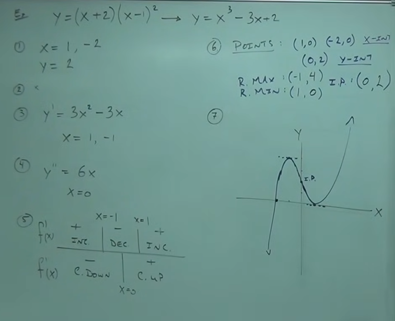
Ａｐｐｌｙｉｎｇ　ｔｈｅ　ｓｔｅｐｓ　ｔｏ　ｔｈｅ　ｉｎｉｔｉａｌ　ｅｘａｍｐｌｅ $𝒇(𝒙)=(𝒙+2)(𝒙-1)^{2}$

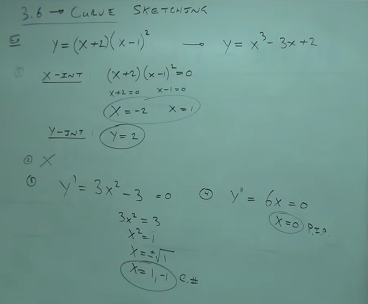
• [1:18]. Step 1: Find the intercepts [image-1]
  • Find 𝒙-intercepts:
    • Set 𝑦 = 0 and solve for 𝒙 (find the roots of the equation).
      • Simplify only if the equation is "easy": quadratic or lower degree, or if it is already factored.
    • $(𝒙+2)(𝒙-1)^{2}=0 \Rightarrow 𝒙+2=0 \;\to\; 𝒙=-2;\; 𝒙-1=0 \;\to\; 𝒙=1$
    • So the x-intercepts are: $𝒙=-2$ and $𝒙=1$.
  • Find the 𝑦-intercept:
    • Set 𝒙 = 0 and solve for 𝑦: $𝒇(0)=(0+2)(0-1)^{2}=2\cdot 1=2$
    • So the y-intercept is: $𝒚=2$.
• Step 2: ❌
• [13:28]. Step 3: First derivative test:
  • Expand the function to make differentiation easier.
    • $𝒇(𝒙)=(𝒙+2)(𝒙-1)^{2}\;\to\; 𝒙^{3}-3𝒙+2$
    • $𝒇'(𝒙)=3𝒙^{2}-3$
  • Solve for critical numbers by setting $𝒇'(𝒙)=0$.
    • $𝒙=\pm 1$.
• [15:05]. Step 4: Second derivative test:
  • $𝒇''(𝒙)=6𝒙$
  • Find the inflection point by setting $𝒇''(𝒙)=0$.
    • $𝒙=0$
• [16:16]. Step 5: Create a table with the critical numbers and the inflection point.
  
• [19:19]. Step 6: Find points.
  • POINTS:
    • 𝒙-Intercepts: $(1,0)$, $(-2,0)$
    • 𝑦-Intercept: $(0,2)$
  • RELATIVE EXTREMA:
    • Relative Maximum (R.MAX): $(-1,4)$
    • Relative Minimum (R.MIN): $(1,0)$
  • INFLECTION POINT:
    • I.P.: $(0,2)$
• [22:23]. Step 7: Plot the points on the Cartesian plane.
  • Analyze intervals of increase and decrease alongside the asymptotes to sketch the graph.

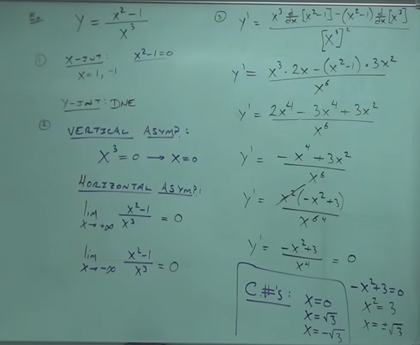
🧩 Ｅｘａｍｐｌｅ　$𝒇(𝒙)=\dfrac{𝒙^{2}-1}{𝒙^{3}}$

• [image-1] [image-2] [image-3] [image-4]
• [28:45]. Step 1: Intercepts:
  • 𝒙-intercepts: Set the numerator equal to zero.
    • $𝒙=1$ and $𝒙=-1$
  • 𝑦-intercept: Set $𝒙=0$.
    • No 𝑦-intercept exists.
• [30:49]. Step 2: Asymptotes:
  • Vertical asymptotes: Set the denominator equal to zero.
    • $𝒙=0$
  • Horizontal asymptotes: Take limits as 𝒙 tends to positive and negative infinity.
    • Divide numerator and denominator by the highest power in the denominator ($𝒙^{3}$).
    • $\displaystyle \lim_{x\to +\infty} 𝒇(𝒙)=0$ and $\displaystyle \lim_{x\to -\infty} 𝒇(𝒙)=0$, so the horizontal asymptote is $y=0$.
• [37:44]. Step 3: First derivative test:
  • Use the quotient rule to differentiate.
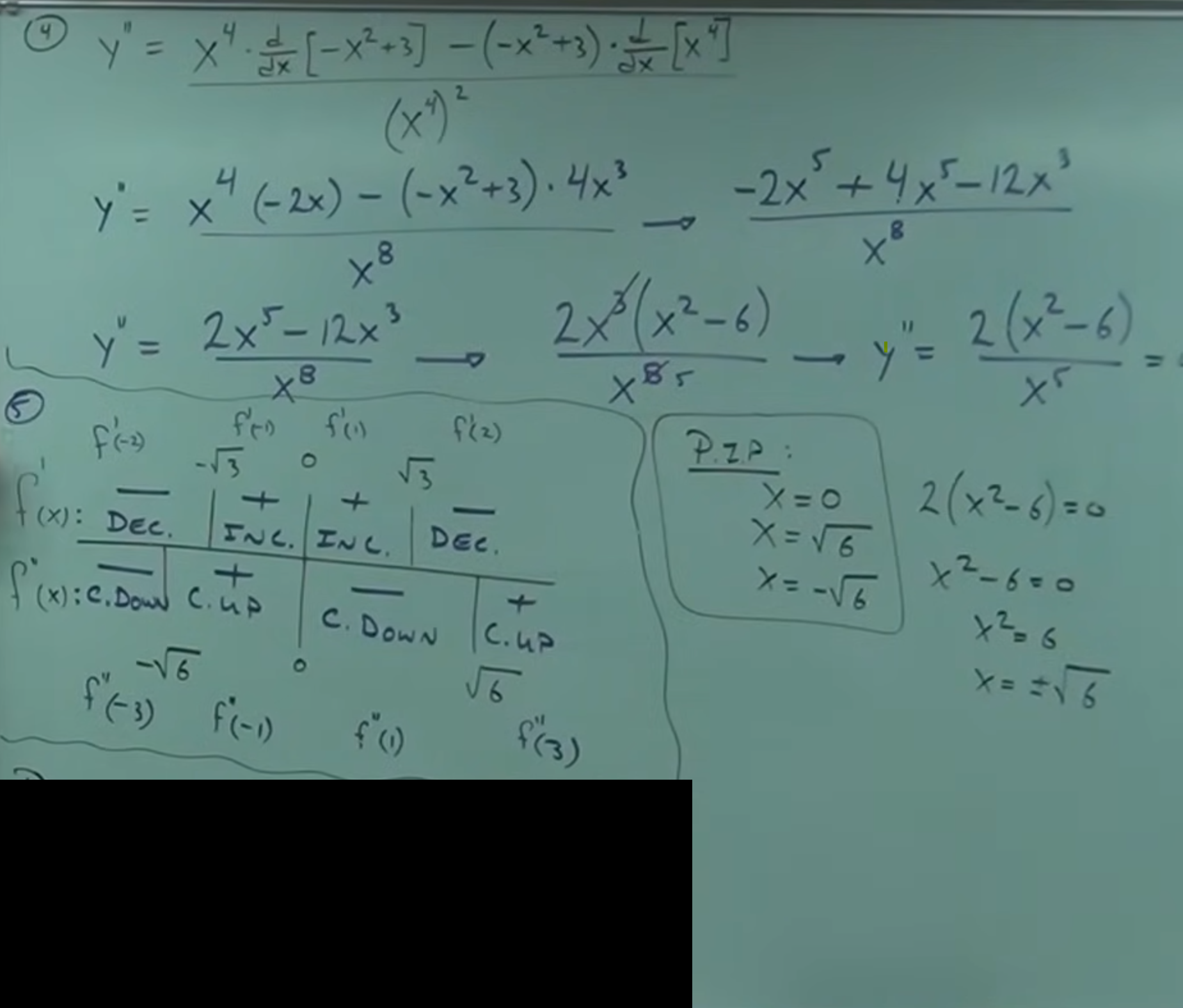
  • Result: $𝒇'(𝒙)=\dfrac{-𝒙^{4}+3𝒙^{2}}{𝒙^{6}}=\dfrac{-𝒙^{2}+3}{𝒙^{4}}$
  • [40:00]. Find critical numbers by setting $𝒇'(𝒙)=0$ and considering where $𝒇'(𝒙)$ is not defined.
    • $𝒙=0,\; 𝒙=\sqrt{3},\; 𝒙=-\sqrt{3}$.
• [42:46]. Step 4: Second derivative test:
  • Result: $𝒇''(𝒙)=\dfrac{2𝒙^{2}-6}{𝒙^{5}}$
  • [45:11]. Find possible inflection points by setting $𝒇''(𝒙)=0$ and considering where $𝒇''(𝒙)$ is not defined.
    • $𝒙=0,\; 𝒙=\sqrt{6},\; 𝒙=-\sqrt{6}$.
• [47:14]. Step 5: Create a table with the critical numbers and the possible inflection points.
  • Test values in each interval to determine the sign of the first and second derivatives.
  
  
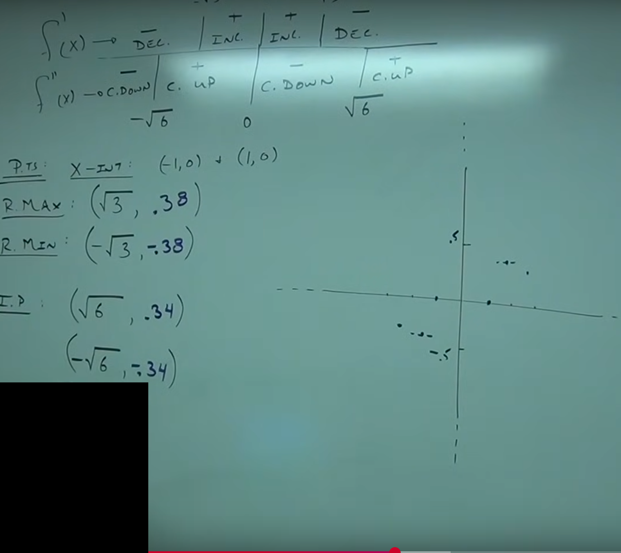
• [57:31]. Step 6: Find the points.
  • Correct the values of the points calculated in class:
    • $(1,0)$ $(-1,0)$
    • R.MAX: $(\sqrt{3},\,0.38)$
    • R.MIN: $(-\sqrt{3},\,-0.38)$
    • IP: $(\sqrt{6},\,0.34)$
    • IP: $(-\sqrt{6},\,-0.34)$
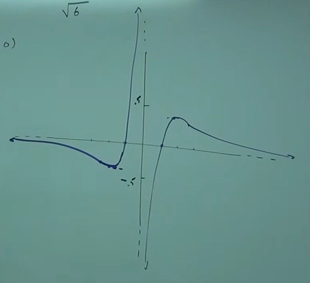
• [58:15]. Step 7: Graph the function.
  • Analyze intervals of increase and decrease alongside the asymptotes to sketch the graph.
  • Conclude that the graph matches the information on concavity.

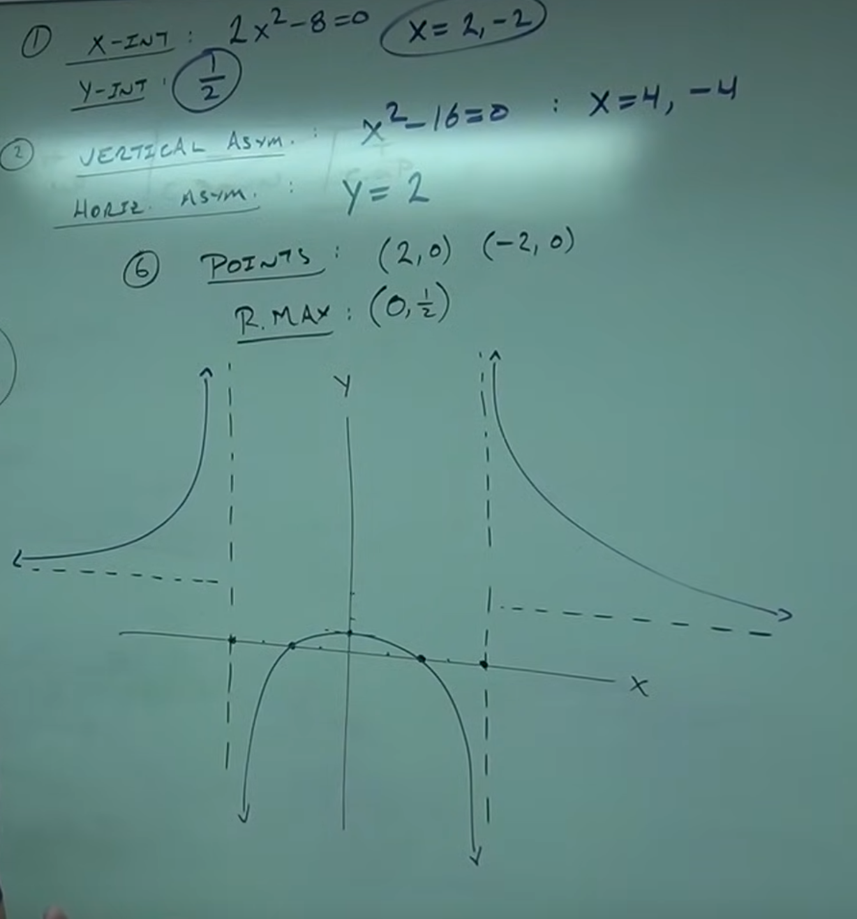
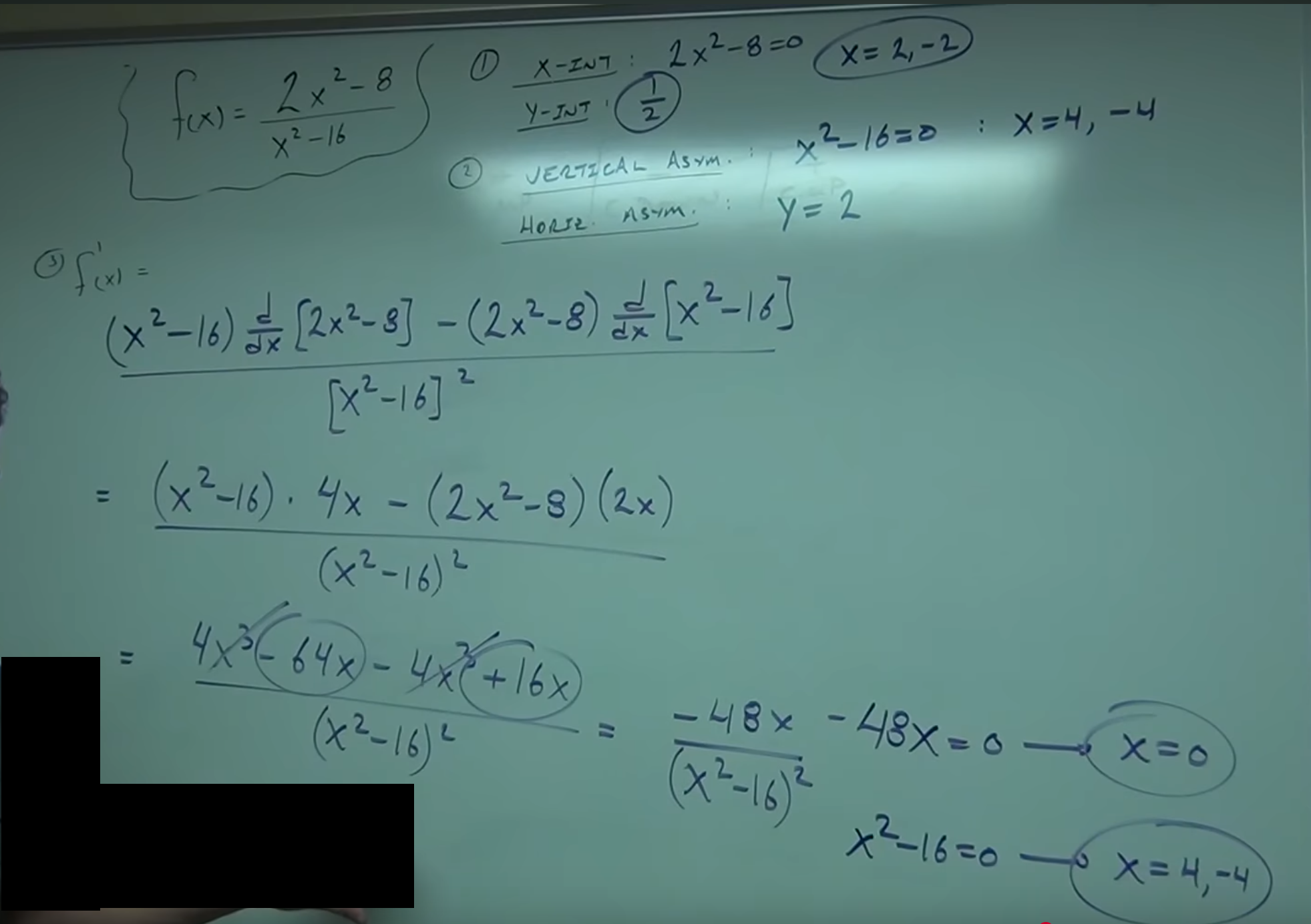
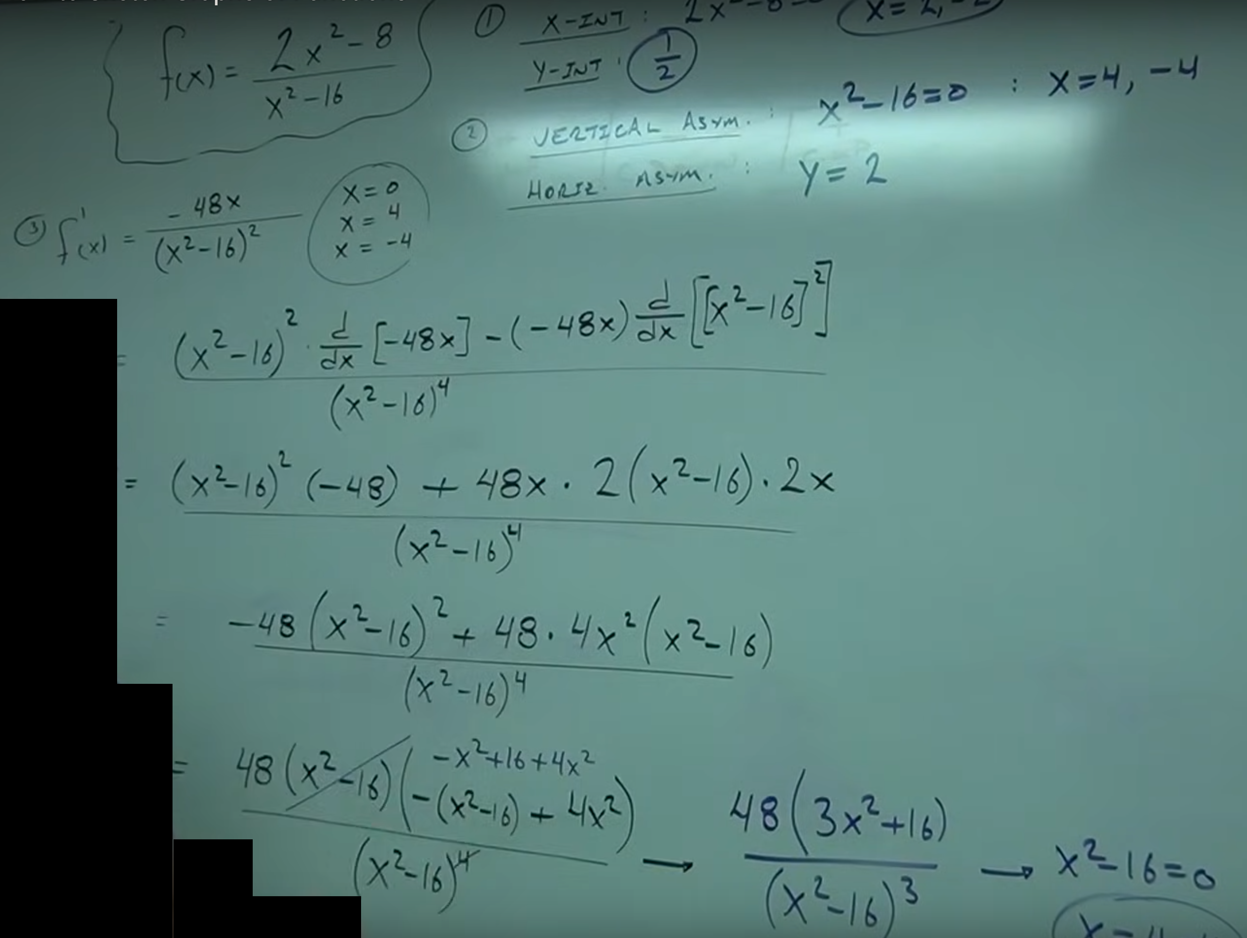
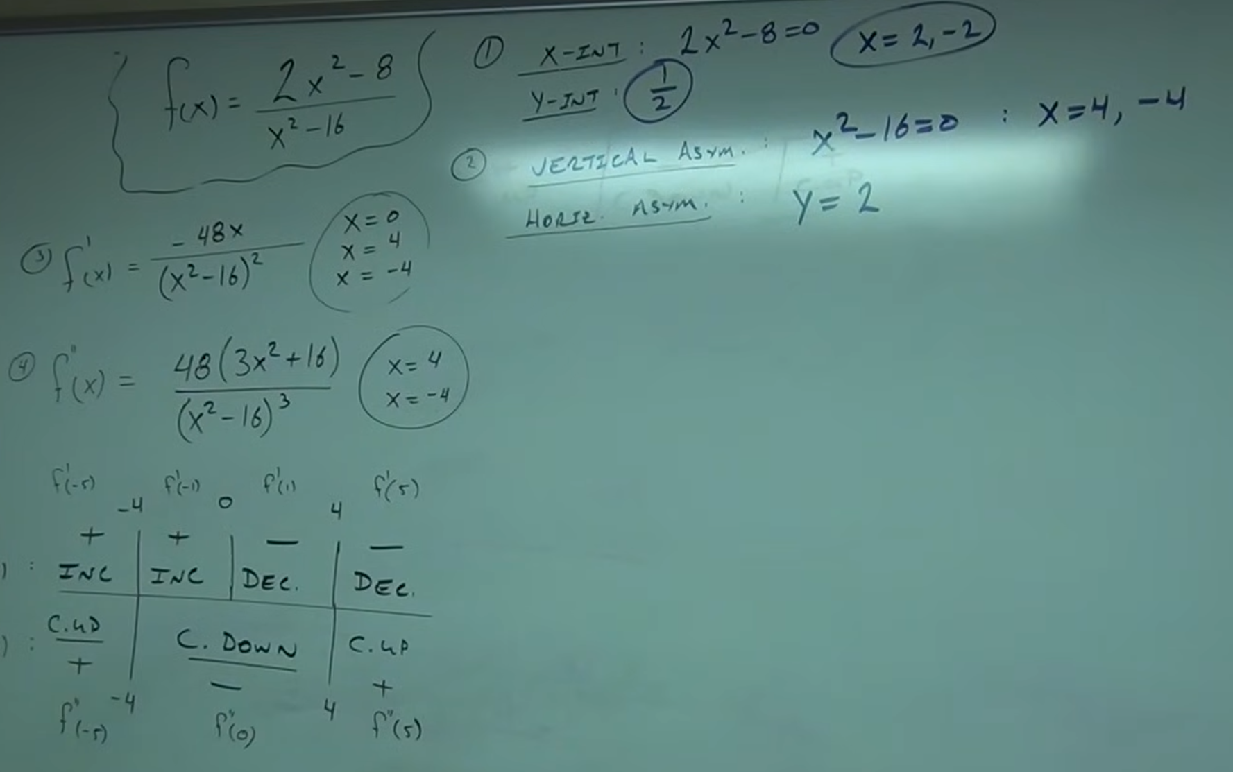
🧩 Ｅｘａｍｐｌｅ　$𝒇(𝒙)=\dfrac{2𝒙^{2}-8}{𝒙^{2}-16}$

• [image-1] [image-2] [image-3] [image-4]
• [1:05:25]. Step 1: Intercepts:
  • 𝒙-intercepts: $2𝒙^{2}-8=0$
    • $𝒙=2$ and $𝒙=-2$
  • 𝑦-intercept: $𝒇(0)$
    • $(0,\dfrac{1}{2})$
• [1:06:26]. Step 2: Asymptotes:
  • Vertical asymptotes: $𝒙^{2}-16=0$
    • $𝒙=4$ and $𝒙=-4$
  • Horizontal asymptotes: $\displaystyle \lim_{x\to +\infty} 𝒇(𝒙)=2$ and $\displaystyle \lim_{x\to -\infty} 𝒇(𝒙)=2$
    • The horizontal asymptote is $y=2$.
• [1:08:22]. Step 3: First derivative test:
  • $𝒇'(𝒙)=\dfrac{-48𝒙}{(𝒙^{2}-16)^{2}}$
  • Find critical numbers by setting $𝒇'(𝒙)=0$ ($-48𝒙=0$)
    • $𝒙=0$
  • Considering where $𝒇'(𝒙)$ is not defined: $(𝒙^{2}-16)^{2}=0$
    • $𝒙=4$, and $𝒙=-4$.
• [1:12:15]. Step 4: Second derivative test:
  • $𝒇''(𝒙)=\dfrac{48(3𝒙^{2}+16)}{(𝒙^{2}-16)^{3}}$
  • Find possible inflection points by setting $𝒇''(𝒙)=0$
    • No inflection points from the numerator.
  • Considering where $𝒇''(𝒙)$ is not defined.
    • The values $𝒙=4$ and $𝒙=-4$ come from the denominator.
• [1:19:19]. Step 5: Create a table with the critical numbers and possible inflection points.
  • Test values in each interval to determine the sign of the first and second derivatives.
  
  
• [1:24:23]. Step 6: Determine the points to plot using previous information.
  • $(2,0)$ $(-2,0)$
  • R.MAX: $(0,\,\dfrac{1}{2})$
  • R.MIN: ❌
  • IP's: ❌
• [1:26:26]. Step 7: Graph the function.