Ｃａｌｃｕｌｕｓ １ Ｌｅｃｔｕｒｅ ４．３

Ａｒｅａ Ｕｎｄｅｒ ａ Ｃｕｒｖｅ， Ｌｉｍｉｔ Ａｐｐｒｏａｃｈ， Ｒｉｅｍａｎｎ Ｓｕｍｓ

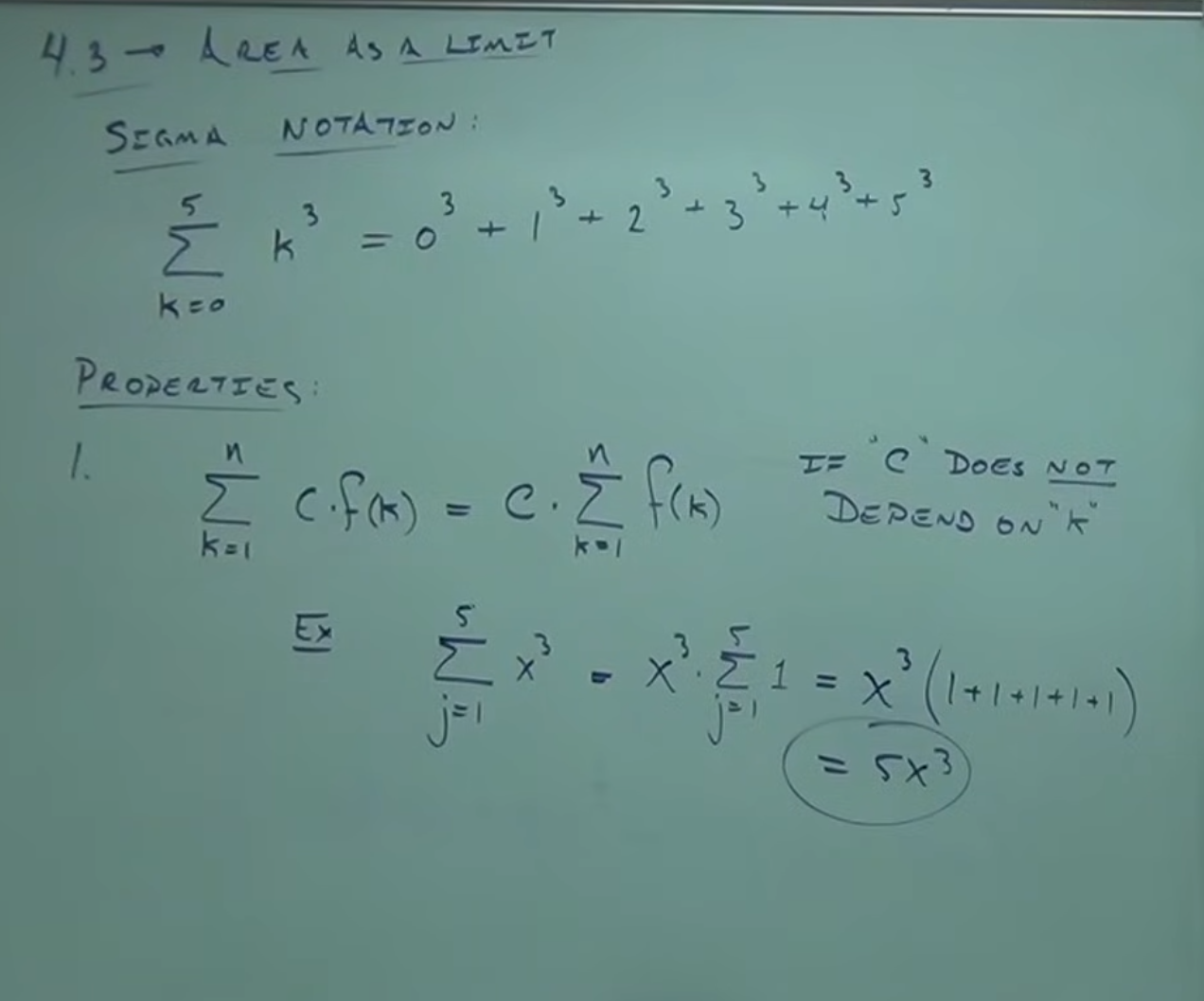
S ｉｇ ｍ ａ　ｎｏｔａｔｉｏｎ

• [0:00]. Introduction to Sigma ( ∑ ) notation.
  • Definition of Sigma as a Greek letter meaning "sum".
• [2:20]. Detailed explanation of Sigma notation.
  • 🧩 Example –: $\displaystyle \sum_{k=0}^{5} k^{3}$
  • Sigma notation indicates the addition of terms.
  • Use of indices (k) and how they vary in the summation is defined.
  • $\displaystyle \sum_{k=0}^{5} k^{3} = 0^{3} + 1^{3} + 2^{3} + 3^{3} + 4^{3} + 5^{3}$
• [3:15]. Summation properties. – [📷image-1] – [📷image-2]
  • [3:30]. Property $\textcolor{magenta}{\text{➀}}$: ᴇxᴛʀᴀᴄᴛɪᴏɴ ᴏꜰ ᴄᴏɴꜱᴛᴀɴᴛꜱ ꜰʀᴏᴍ ᴛʜᴇ ꜱᴜᴍᴍᴀᴛɪᴏɴ.
    • If a constant 𝓬 does not depend on k, the constant factor in the summation can be pulled out.
      • $\displaystyle \sum_{k=1}^{n}\!\big[\;𝓬\cdot 𝒇(k)\;\big]=𝓬\cdot \sum_{k=1}^{n} 𝒇(k)$
      • Special case: $\displaystyle \sum_{k=1}^{n} 𝓬 = 𝓬\cdot n$
    • [5:27]. 🧩 Example –: $\displaystyle \sum_{j=1}^{5} 𝒙^{3}$
      • $\,𝒙^{3}\cdot \sum_{j=1}^{5} 1 = 𝒙^{3}\cdot(1+1+1+1+1)=5\cdot 𝒙^{3}$
  • [9:00]. Property $\textcolor{cyan}{\text{➁}}$: ᴅɪꜱᴛʀɪʙᴜᴛɪᴠᴇ ᴩʀᴏᴩᴇʀᴛy ᴏꜰ ꜱᴜᴍᴍᴀᴛɪᴏɴ ᴏᴠᴇʀ ᴀᴅᴅɪᴛɪᴏɴ ᴀɴᴅ ꜱᴜʙᴛʀᴀᴄᴛɪᴏɴ.
    • Just like derivatives and integrals, the summation can split sums and differences into separate summations.
      • $\displaystyle \sum_{k=1}^{n}\!\big[𝒇(k)+𝓰(k)\big]=\sum_{k=1}^{n} 𝒇(k)+\sum_{k=1}^{n} 𝓰(k)$
      • 🧩 Example –: $\displaystyle \sum_{k=1}^{3}\!\big[k+2k\big]=\sum_{k=1}^{3}k+\sum_{k=1}^{3}2k$
• [9:35]. ꜰᴏʀᴍᴜʟᴀꜱ ꜰᴏʀ ꜱᴜɪᴍᴍᴀᴛɪᴏɴ ᴍᴀɴɪᴩᴜʟᴀᴛɪᴏɴ – [📷image]
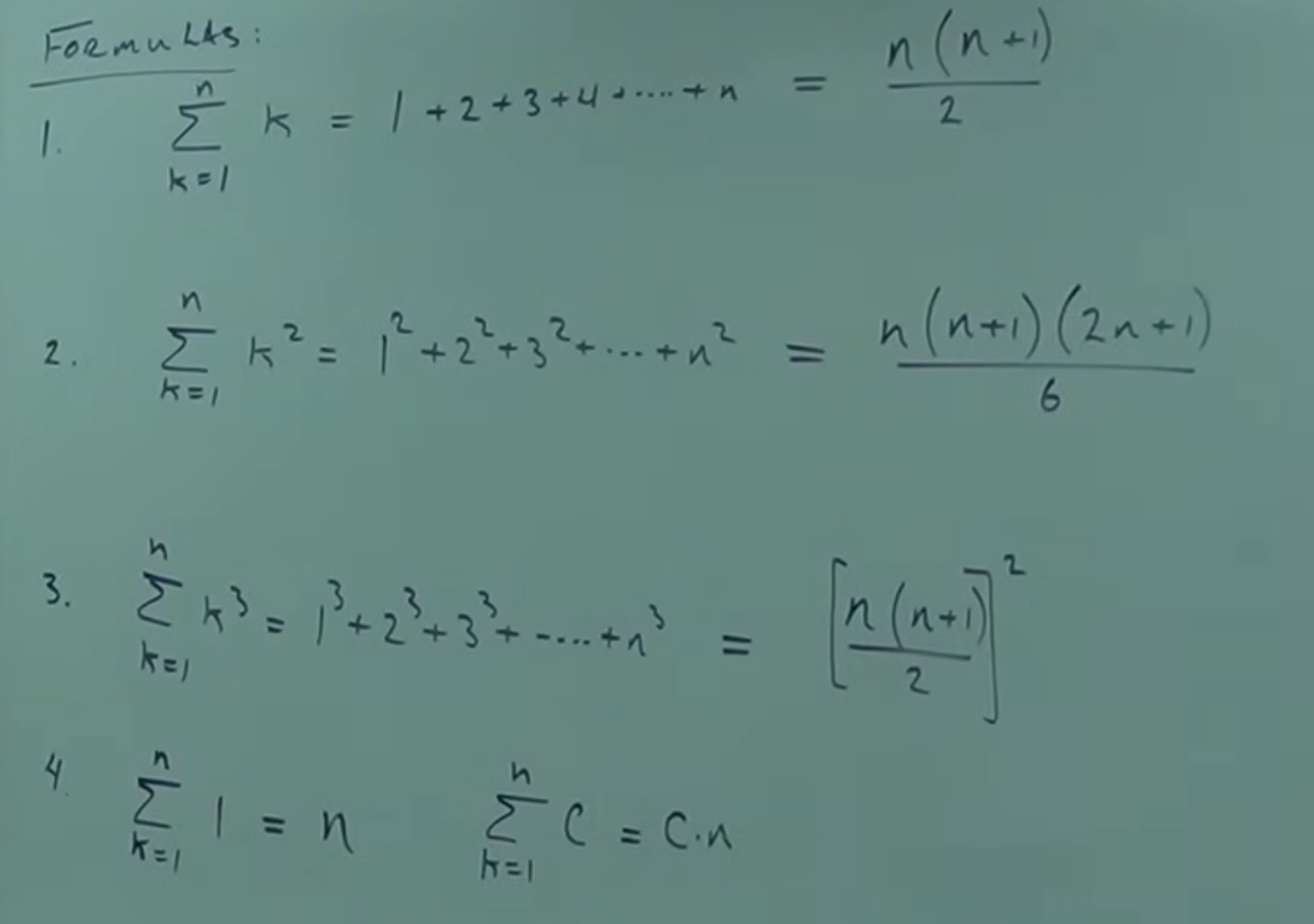
  • ❶ $\displaystyle \sum_{k=1}^{n} k = 1+2+3+4+\dots+n=\dfrac{n(n+1)}{2}$
  • ❷ $\displaystyle \sum_{k=1}^{n} k^{2}=1^{2}+2^{2}+3^{2}+\dots+n^{2}=\dfrac{n(n+1)(2n+1)}{6}$
  • ❸ $\displaystyle \sum_{k=1}^{n} k^{3}=1^{3}+2^{3}+3^{3}+\dots+n^{3}=\left(\dfrac{n(n+1)}{2}\right)^{2}$
  • ❹ $\displaystyle \sum_{k=1}^{n} 1=n\ ;\ \sum_{k=1}^{n} 𝓬=\underbrace{𝓬+𝓬+\dots+𝓬}_{n\ \text{terms}}=𝓬\cdot \underbrace{(1+1+\dots+1)}_{n}=𝓬\cdot n$
• [17:15]. 🧩 Example – Applying summation formulas: $\displaystyle \sum_{k=1}^{10}\big[k(k+1)\big]$ – [📷image]
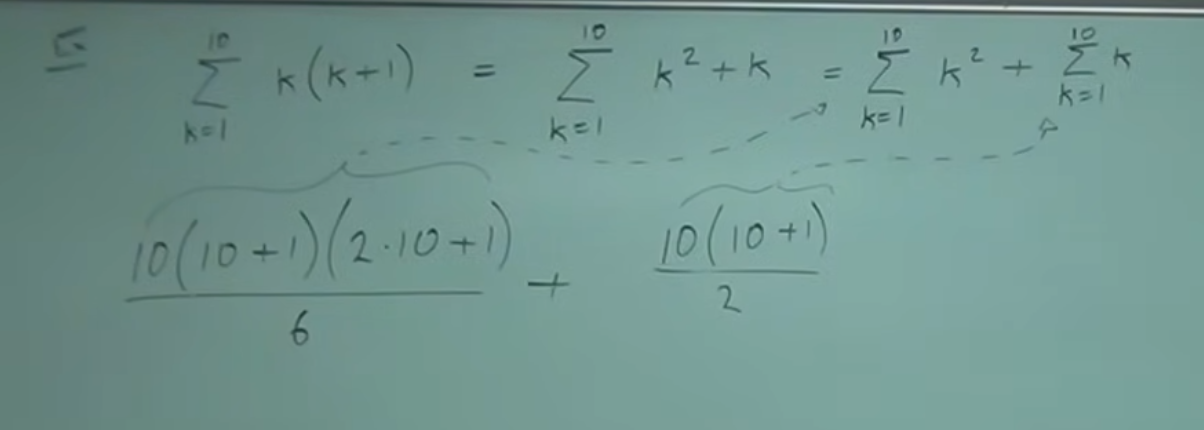
  • The need to manipulate sums in order to use the above formulas.
  • The idea of distributing products of terms so the formulas can be applied is presented.
  • It is explained that summations can be separated through addition or subtraction.
  • $\displaystyle \sum_{k=1}^{10}\big[k(k+1)\big]=\sum_{k=1}^{10}\!\big[k^{2}+k\big]=\sum_{k=1}^{10}k^{2}+\sum_{k=1}^{10}k\ \,$ $\textcolor{cyan}{\text{➁}}$
  • Applied formulas:
    $\displaystyle \sum_{k=1}^{n} k^{2}= \dfrac{n(n+1)(2n+1)}{6}$ ❷
    $\displaystyle \sum_{k=1}^{n} k= \dfrac{n(n+1)}{2}$ ❶
    Substituting $n=10$:
    $\displaystyle \dfrac{10(10+1)(2\cdot 10+1)}{6}+\dfrac{10(10+1)}{2}=\dfrac{10\cdot 11\cdot 21}{6}+\dfrac{10\cdot 11}{2}=385+55=440$

Ｃａｌｃｕｌａｔｉｎｇ　ｔｈｅ　ａｒｅａ　ｕｎｄｅｒ　ａ　ｃｕｒｖｅ　ｕｓｉｎｇ　ｒｅｃｔａｎｇｌｅｓ

• [23:15]. Definition of the rectangular method. – [📷image]
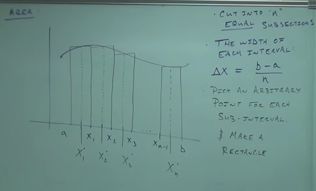
  • How the area under the curve is split into $n$ equal subdivisions is explained.
  • Partition of the interval $[𝓪,𝓫]$ into $n$ equal subintervals.
    • Equal-width subintervals simplify the algebra and notation.
    • Define the cut points (partition): $𝒙_{0}, 𝒙_{1}, 𝒙_{2},\dots, 𝒙_{n}$ with $𝒙_{0}=𝓪$ and $𝒙_{n}=𝓫$.
    • These cuts determine $n$ adjacent subintervals $[𝒙_{k-1}, 𝒙_{k}]$ and hence $n$ rectangles.
      • and $k\in\{1,2,\dots,n\}$ (index)
  • [25:02]. The width of each rectangle is defined as $\Delta 𝒙$.
    • $\Delta 𝒙$ is the change in $𝒙$ from one point to the next, for example from $𝓪$ to $𝒙_{1}$.
    • It is shown how to calculate the width of the rectangles by:
      • $\,𝓫-𝓪$
    • The formula for the width of each rectangle is given:
      • $\displaystyle \Delta 𝒙=\dfrac{𝓫-𝓪}{n}$
    • It is pointed out that all the rectangle bases are the same, simplifying their sum.
  • [28:05]. Choice of sample points to determine the heights.
    • In each subinterval $[𝒙_{k-1}, 𝒙_{k}]$, pick an arbitrary sample point $x_{k}^{\ast}\in[𝒙_{k-1}, 𝒙_{k}]$
      • Examples: a point in $[𝓪, 𝒙_{1}]$ or in $[𝒙_{3}, 𝒙_{4}]$
    • The height of the $k$-th rectangle is $𝒇(x_{k}^{\ast})$
      • With that height $h_{k}$, you build ONE rectangle that spans the entire subinterval:
        • base $=\Delta 𝒙 = 𝒙_{k}-𝒙_{k-1}$ (constant if the partition is uniform)
        • height $=h_{k}=f(x_{k}^{\ast})$ (constant across the whole subinterval)
        • area of the $k$-th rectangle: $\mathcal{A}_{k}=f(x_{k}^{\ast})\cdot \Delta 𝒙$
  • It is explained that to sum the areas of all rectangles, one can consider each rectangle individually.
    • The sum of the $n$ rectangle areas approximates the area under the curve.
  • It is explained that the area under the curve is approximated by summing the rectangles’ areas.
    • The approximation improves as $n$ increases ($\Delta 𝒙\to 0$).
  • 🗒️NOTE: Remarks on choices of $x_{k}^{\ast}$ (special cases used in practice).
    • Left endpoints: $x_{k}^{\ast}=𝒙_{k-1}$ (left Riemann sum).
    • Right endpoints: $x_{k}^{\ast}=𝒙_{k}$ (right Riemann sum).
    • Midpoints: $x_{k}^{\ast}=\dfrac{𝒙_{k-1}+𝒙_{k}}{2}$ (often more accurate for smooth $𝒇$).
• [34:24]. Analysis of the area of an individual rectangle. – [📷image]
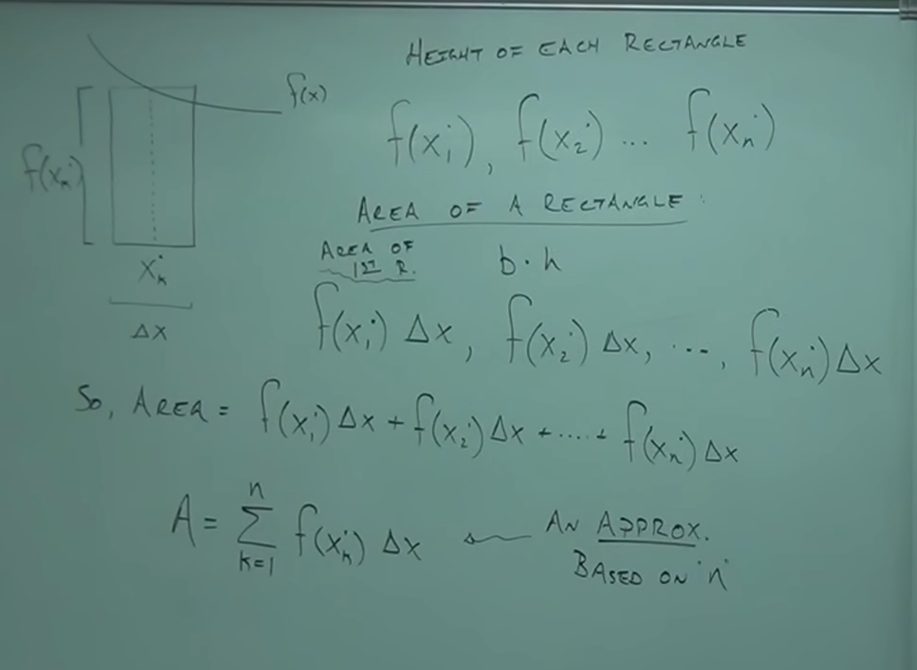
  • [36:10]. Rectangle base (width): $\displaystyle \Delta 𝒙=\dfrac{𝓫-𝓪}{n}$ for uniform partitions.
  • The idea of using an arbitrary point $x_{k}^{\ast}$ to get the rectangles’ heights is presented.
  • [39:00]. To get each rectangle’s height, $𝒇(x_{k}^{\ast})$ is evaluated at that arbitrary point.
  • [41:20]. It follows that the area of a rectangle is its base times height: $\Delta 𝒙\cdot 𝒇(x_{k}^{\ast})$.
  • [42:36]. The sum of the areas of all individual rectangles.
    • $\mathcal{A}=\displaystyle \sum_{k=1}^{n} 𝒇(x_{k}^{\ast})\cdot \Delta 𝒙.$
  • 🗒️NOTE: Summary of definitions (clean reference).
    • Partition: $\mathcal{P}=\{\,𝒙_{0}=𝓪<𝒙_{1}<\dots<𝒙_{n}=𝓫\,\}$.< /li>
    • Widths: $\displaystyle \Delta 𝒙=\dfrac{(𝓫-𝓪)}{n}$
    • Sample points: $x_{k}^{\ast}\in[𝒙_{k-1}, 𝒙_{k}]$.
    • Riemann sum: $\displaystyle \sum_{k=1}^{n} 𝒇(x_{k}^{\ast})\cdot \Delta 𝒙$
• [46:50]. Improving the approximation using limits.
  • It is explained that to improve the approximation, the number of rectangles must increase.
    • $\mathcal{A}_{n}=\displaystyle \sum_{k=1}^{n} 𝒇(x_{k}^{\ast})\cdot \Delta 𝒙 \ \rightsquigarrow\ \mathcal{A}_{n}$ approximation based on $n$
      • Index and points:
        • $k\in\{1,2,\dots,n\}$
        • $x_{0}=𝓪,\ x_{n}=𝓫,\ \text{with } 𝓪=x_{0}
        • $x_{k}^{\ast}\in[x_{k-1},x_{k}]$
  • If the number of rectangles tends to infinity, the approximation is exact.
  • When the number of rectangles increases, each rectangle’s width shrinks, tending to zero.
  • The concept of the limit is introduced to handle $n\to\infty$.
  • It is stated that to let $n\to\infty$, one uses the limit operation.
  • [48:50]. It is established that applying the limit to the sum of the rectangles’ areas yields the exact area under the curve.
    • $\mathcal{A}_{n}=\displaystyle \lim_{n\to\infty}\sum_{k=1}^{n} 𝒇(x_{k}^{\ast})\cdot \Delta 𝒙$
    • It is stated that the limit of a sum is the foundation of the integral.
      • $\displaystyle \mathcal{A}_{n}=\lim_{n\to\infty}\sum_{k=1}^{n} 𝒇(x_{k}^{\ast})\cdot \Delta 𝒙\ \longrightarrow\ \int_{𝓪}^{𝓫} 𝒇(x)\,dx$
      • $[𝓪,𝓫]$ are the limits of the interval (Definite Integral because of $[𝓪,𝓫]$) over which the integral is evaluated.

Ｈｏｗ　ｔｏ　ｕｓｅ　ｔｈｅ　ｄｅｆｉｎｉｔｅ　ｉｎｔｅｇｒａｌ　ｔｏ　ｆｉｎｄ　ａｒｅａｓ

• [50:50]. Arbitrary point’s of each subinterval. – [📷image]
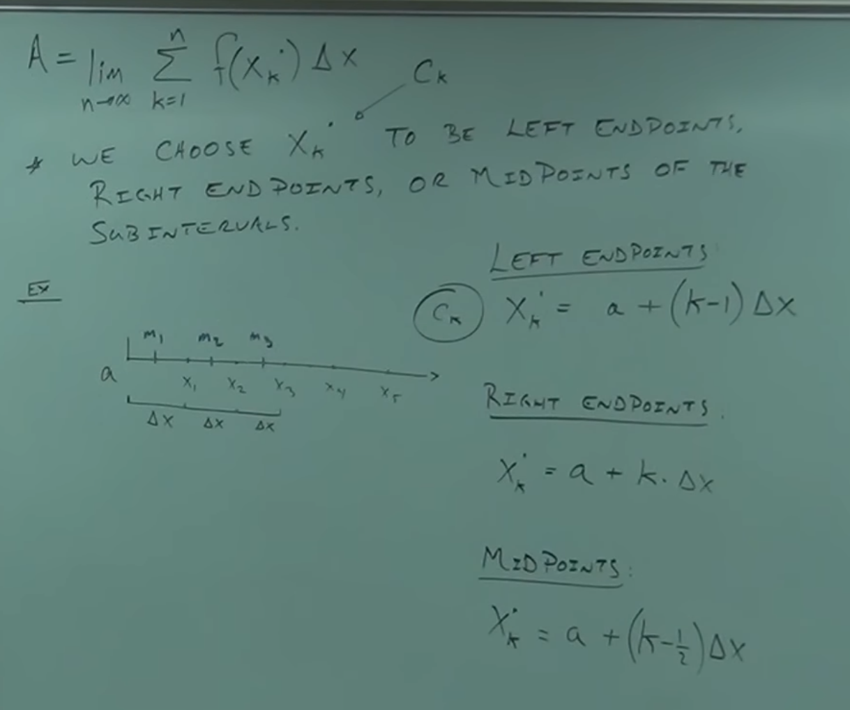
  • It is explained that the arbitrary point $x_{k}^{\ast}$ can be any point in the subinterval.
  • The arbitrary point’s position does not matter, as the rectangle width tends to zero.
  • For convenience, one typically chooses consistently the left endpoint, right endpoint, or midpoint.
  • Choosing arbitrary points: Left, Right, and Midpoint.
    • $x_{k}^{\ast}$ can represent the left, right, or midpoint of the subinterval.
  • [53:55]. Visualizing the cut points on the $𝒙$-axis.
    • To calculate the area, one needs a finite interval from $𝓪$ to $𝓫$
    • The cuts on the $𝒙$-axis are set as $𝒙_{1}, 𝒙_{2}, 𝒙_{3}, \dots, 𝒙_{n}$.
    • The width of each rectangle is $\Delta 𝒙$.
    • There is an arbitrary point at each cut.
    • Visualizing the different options for the arbitrary point
      • For left-end selection, the arbitrary point is the left endpoint of each subinterval.
    • Left endpoints: $x_{k}^{\ast}=𝒙_{k-1}$ (left Riemann sum).
      • For right-end selection, the arbitrary point is the right endpoint of each subinterval.
    • Right endpoints: $x_{k}^{\ast}=𝒙_{k}$ (right Riemann sum).
      • For midpoint selection, the arbitrary point is the midpoint of each subinterval.
    • Midpoints: $x_{k}^{\ast}=\dfrac{𝒙_{k-1}+𝒙_{k}}{2}$ (often more accurate for smooth $𝒇$).

      •                      xₖ₋₁       xₖ*         xₖ
                             │----------│----------│  ← base = Δx; k∈{1,2,…,n}
                                        ▲
                                        │ 𝒇(xₖ*)  
                            

    • According to the choice.
      • A formula is needed to calculate each arbitrary point.
      • The goal is to find a formula for $x_{k}^{\ast}$ so it can be substituted into $𝒇(x_{k}^{\ast})$.
        • $\displaystyle \mathcal{A}_{n}=\lim_{n\to\infty}\sum_{k=1}^{n} 𝒇(x_{k}^{\ast})\cdot \Delta 𝒙$
      • It is explained that the formula for $x_{k}^{\ast}$ will give a value in terms of $𝒙$ and $k$.
      • The result allows one to handle the sum and the limit.
  • [57:20]. The formula for each arbitrary points $x_{k}^{\ast}$ must start with $𝓪$
    • $x_{k}^{\ast}=𝓪\ \dots$
• [58:20]. Arbitrary points using the right endpoint.
  • It is explained that for right endpoints, the first arbitrary point is $𝓪+\Delta 𝒙$, not just $𝓪$.
  • The second arbitrary point is $𝓪+2\cdot \Delta 𝒙$.
  • For the $n$th point, the distance from $𝓪$ is $n\cdot \Delta 𝒙$.
  • The formula for $x_{k}^{\ast}$ using the right endpoint is $x_{k}^{\ast}= 𝒙_{k}=𝓪+k\cdot \Delta 𝒙$.
• [1:0:17]. Arbitrary points using the left endpoint.
  • It is explained that for left endpoints, the first arbitrary point is $𝓪$.
  • The second arbitrary point is $𝓪+\Delta 𝒙$.
  • The formula for $x_{k}^{\ast}$ using the left endpoint is $x_{k}^{\ast}=𝒙_{k-1}=𝓪+(k-1)\cdot \Delta 𝒙$.
  • It is noted that, compared to the right endpoints, one starts one subinterval earlier.
• [1:02:35]. Arbitrary points using the midpoint.
  • It is stated that for midpoints, one must compute half the width of each subinterval.
  • The general formula for the midpoint is $x_{k}^{\ast}=\dfrac{𝒙_{k-1}+𝒙_{k}}{2}=𝓪+\big(k-\tfrac12\big)\cdot \Delta 𝒙$
  • Midpoints often provide a better approximation even with fewer rectangles, especially for smooth functions.
• Summary of formulas for arbitrary points.

  Method	Formula for 𝒙ₖ*	Equivalent form
  Left Endpoints	$x_{k}^{\ast}=𝓪+(k-1)\Delta 𝒙$	$𝒙_{k-1}$
  Right Endpoints	$x_{k}^{\ast}=𝓪+k\Delta 𝒙$	$𝒙_{k}$
  Midpoints	$x_{k}^{\ast}=𝓪+\big(k-\tfrac12\big)\Delta 𝒙$	$\dfrac{𝒙_{k-1}+𝒙_{k}}{2}$

Ｉｎｔｒｏｄｕｃｔｉｏｎ　ｔｏ　ｔｈｅ　ｐｒａｃｔｉｃａｌ　ａｐｐｌｉｃａｔｉｏｎ　ｏｆ　ｔｈｅ　ｍｅｔｈｏｄ

• [1:04:26]. A practical example is necessary to understand the method’s concept.
  • The idea is to sum the areas of small rectangles and then apply the limit.
  • The concept of limits is the foundation of calculus.
• [1:05:50]. 🧩 Example –1: Calculating the area under $𝒇(𝒙)=𝒙^{2}$ on $[0,1]$ using right endpoints. – [📷image-1] – [📷image-2]
  • In real life one could pick any arbitrary point, and all choices yield the same final result.
  • Right endpoints are used here.
  • It is mentioned that right endpoints are often easier to handle than left endpoints.
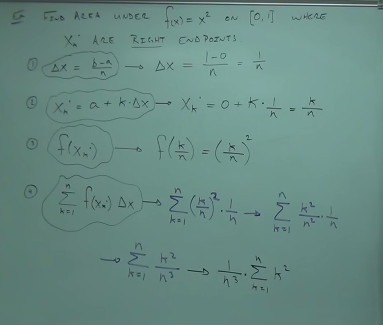
  • The first step is to calculate $\Delta 𝒙$.
  • [1:06:55]. Step 1: Calculate $\Delta 𝒙$
    • The formula $\displaystyle \Delta 𝒙=\dfrac{𝓫-𝓪}{n}$ is stated.
    • With $𝓪=0$ and $𝓫=1$, it follows that $\Delta 𝒙=\dfrac{1}{n}$
  • [1:09:05]. Step 2: Calculate $x_{k}^{\ast}$
    • Recall the formula for the right endpoint: $x_{k}^{\ast}=𝓪+k\cdot \Delta 𝒙$.
    • Substituting $𝓪=0$ and $\Delta 𝒙=\dfrac{1}{n}$ gives $x_{k}^{\ast}=\dfrac{k}{n}$
  • [1:10:50]. Step 3: Calculate $𝒇(x_{k}^{\ast})$.
    • It is recalled that $x_{k}^{\ast}$ must be substituted into the function $𝒇(𝒙)$.
    • Substituting $x_{k}^{\ast}=\dfrac{k}{n}$ into $𝒇(𝒙)=𝒙^{2}$ gives $𝒇(x_{k}^{\ast})=\left(\dfrac{k}{n}\right)^{2}$
    • If there were a constant added to $x_{k}^{\ast}$, the problem would be more difficult.
    • It is noted that this can be done using the integral as well.
  • [1:13:00]. Step 4: Build the summation.
    • The approximation for the area is given by $\displaystyle \sum_{k=1}^{n}\big[𝒇(x_{k}^{\ast})\cdot \Delta 𝒙\big]$
    • The previously calculated values are substituted.
      • $\displaystyle \sum_{k=1}^{n} \dfrac{k^{2}}{n^{3}}$
    • This expression must be algebraically manipulated to be evaluated.
    • Manipulating the summation.
      • The property of summation is used to separate constants.
      • It is noted that $k^{2}$ is a variable term and $n^{3}$ is constant in the summation, so $n^{3}$ can be factored out.
      • This property is why the earlier steps were carried out.
        • $\displaystyle \sum_{k=1}^{n} \dfrac{k^{2}}{n^{3}} \ \to\ \dfrac{1}{n^{3}}\cdot \sum_{k=1}^{n} k^{2}$
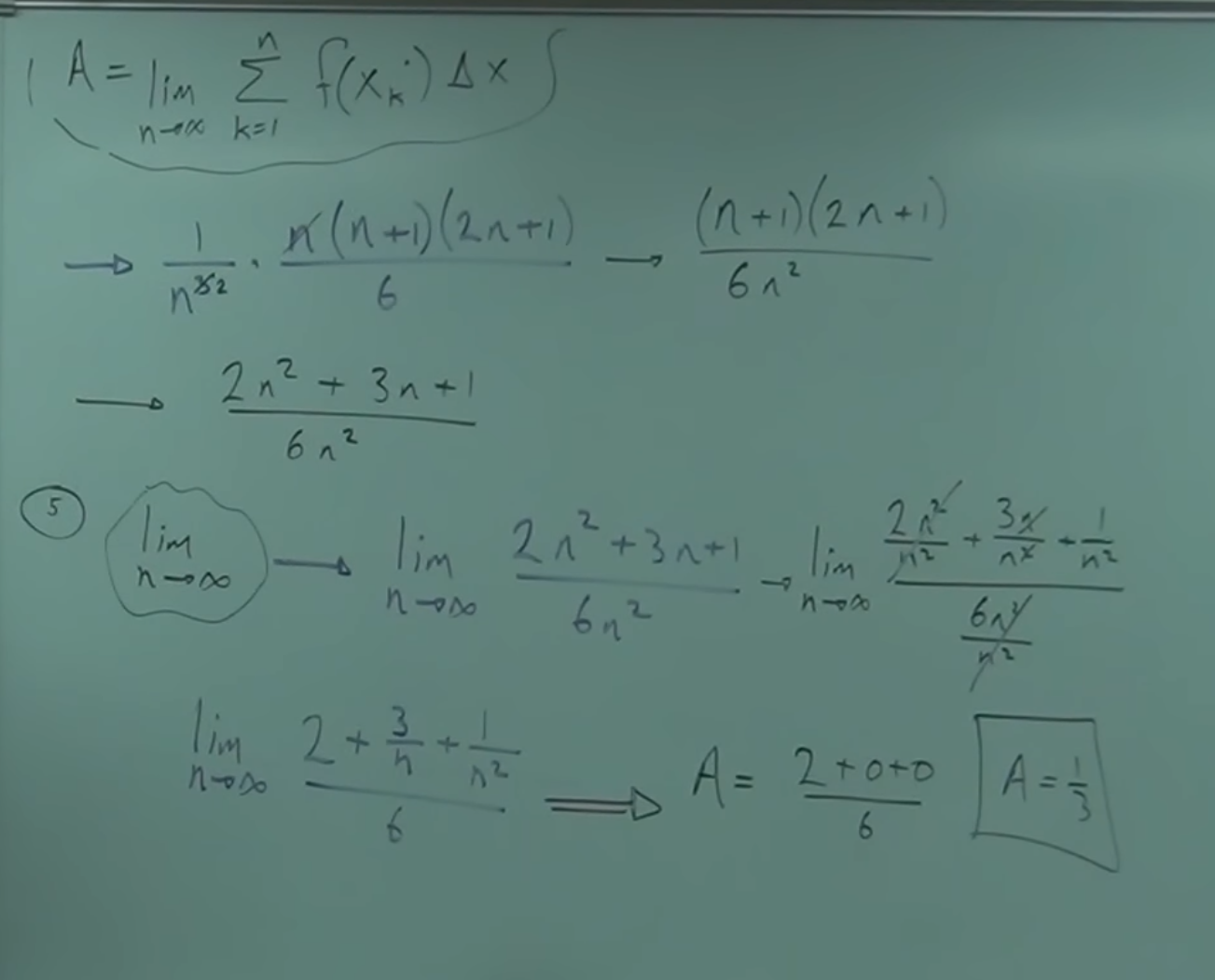
      • The formula for summing $k^{2}$ is applied: $\displaystyle \sum_{k=1}^{n} k^{2}=\dfrac{n(n+1)(2n+1)}{6}$
      • hence: $\displaystyle \sum_{k=1}^{n} \dfrac{k^{2}}{n^{3}}=\dfrac{2n^{2}+3n+1}{6n^{2}}$
  • [1:17:30]. Step 5: Calculate the limit.
    • After evaluating the summation, $\displaystyle \lim_{n\to\infty}$ can be computed.
    • It is noted that such a limit yields a finite value since the area under the curve is finite.
    • The limit is applied to the previously obtained algebraic expression.
    • The method for solving limits at infinity for rational functions is recalled.
    • By applying these properties, the result $\dfrac{1}{3}$ is obtained.
      • $\displaystyle \lim_{n\to\infty}\dfrac{2n^{2}+3n+1}{6n^{2}}=\dfrac{1}{3}$
    • It is concluded that the area under $𝒇(𝒙)=𝒙^{2}$ on $[0,1]$ is $\dfrac{1}{3}$.

Ｄｉｓｃｕｓｓｉｏｎ　ｏｎ　ｔｈｅ　ｃｏｎｃｅｐｔ　ｏｆ　“ｓｉｇｎｅｄ　ｎｅｔ　ａｒｅａ”

• [1:22:40]. The concept of “signed net area”. – [📷image]
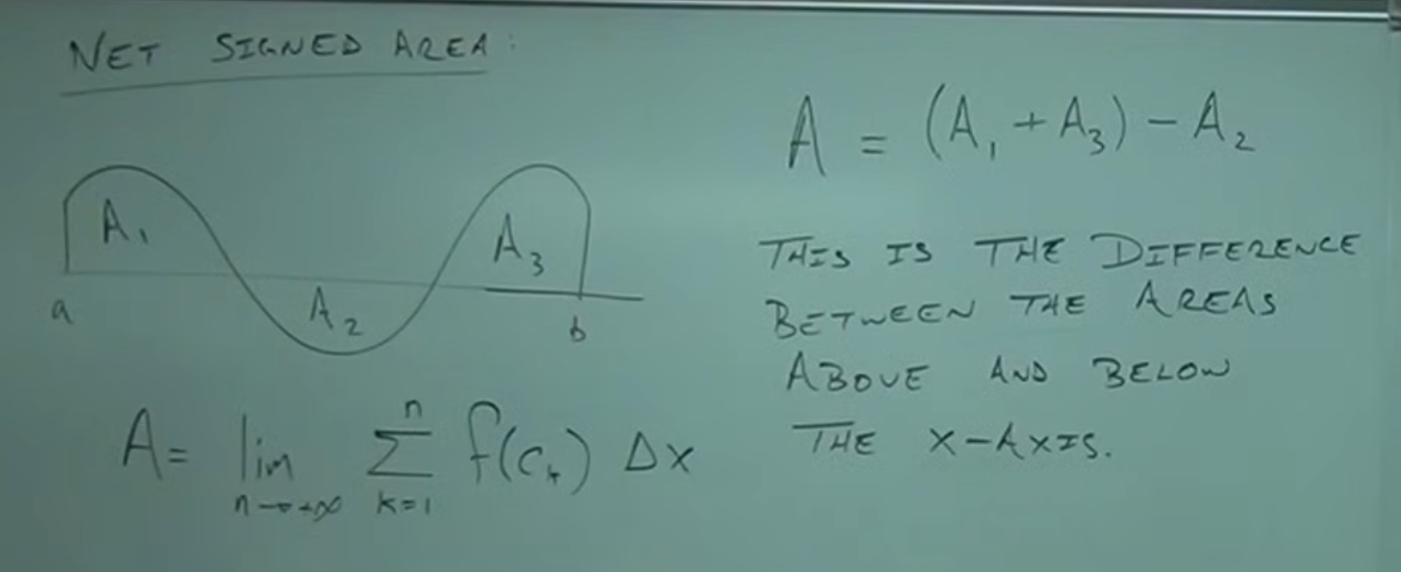
  • The concept of “signed net area” is introduced as the result of the integration method.
  • Up to this point, the examples considered functions entirely above the $𝒙$-axis.
  • When the function dips below the $𝒙$-axis:
    • The integral assigns positive area to regions above the axis.
    • The integral assigns negative area to regions below the axis.
  • The net area is obtained by combining both contributions:
    • $\mathcal{A}=\mathcal{A}_{\text{above}}-\mathcal{A}_{\text{below}}$
    • This means the integral computes the difference, not the total geometric area.
  • Important clarification:
    • Symmetry alone does not determine the sign of the result.
    • The computed value is always the signed net area, which incorporates the idea of orientation relative to the $𝒙$-axis.
  • 🧩 Example –: $\displaystyle \int_{-1}^{1} x\,dx$
    • The graph of $f(x)=x$ is symmetric about the origin.
    • The area from $[0,1]$ is positive: $\displaystyle \int_{0}^{1} x\,dx=\dfrac{1}{2}$.
    • The area from $[-1,0]$ is negative: $\displaystyle \int_{-1}^{0} x\,dx=-\dfrac{1}{2}$.
    • Adding them: $\dfrac{1}{2}+(-\dfrac{1}{2})=0$.
    • The total area (geometric) is $1$, but the net signed area is $0$.
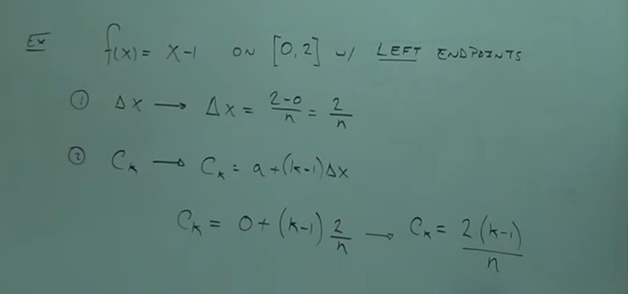
• [1:27:20]. 🧩 Example – 2: Calculating the net area under $𝒇(𝒙)=𝒙-1$ on $[0,2]$ using left endpoints. – [📷image-1] – [📷image-2] – [📷image-3]
  • [1:27:50]. Step 1: Calculate $\Delta 𝒙$
    • The formula $\displaystyle \Delta 𝒙=\dfrac{𝓫-𝓪}{n}$ is noted
    • With $𝓪=0$ and $𝓫=2$, it follows that $\Delta 𝒙=\dfrac{2}{n}$
  • [1:28:20]. Step 2: Calculate $x_{k}^{\ast}$
    • Recall the formula for the left endpoint: $x_{k}^{\ast}=𝓪+(k-1)\cdot \Delta 𝒙$
    • Substituting $𝓪=0$ and $\Delta 𝒙=\dfrac{2}{n}$ yields $x_{k}^{\ast}=\dfrac{2(k-1)}{n}$
    • It is recommended not to distribute $2/n$ for easier subsequent operations.
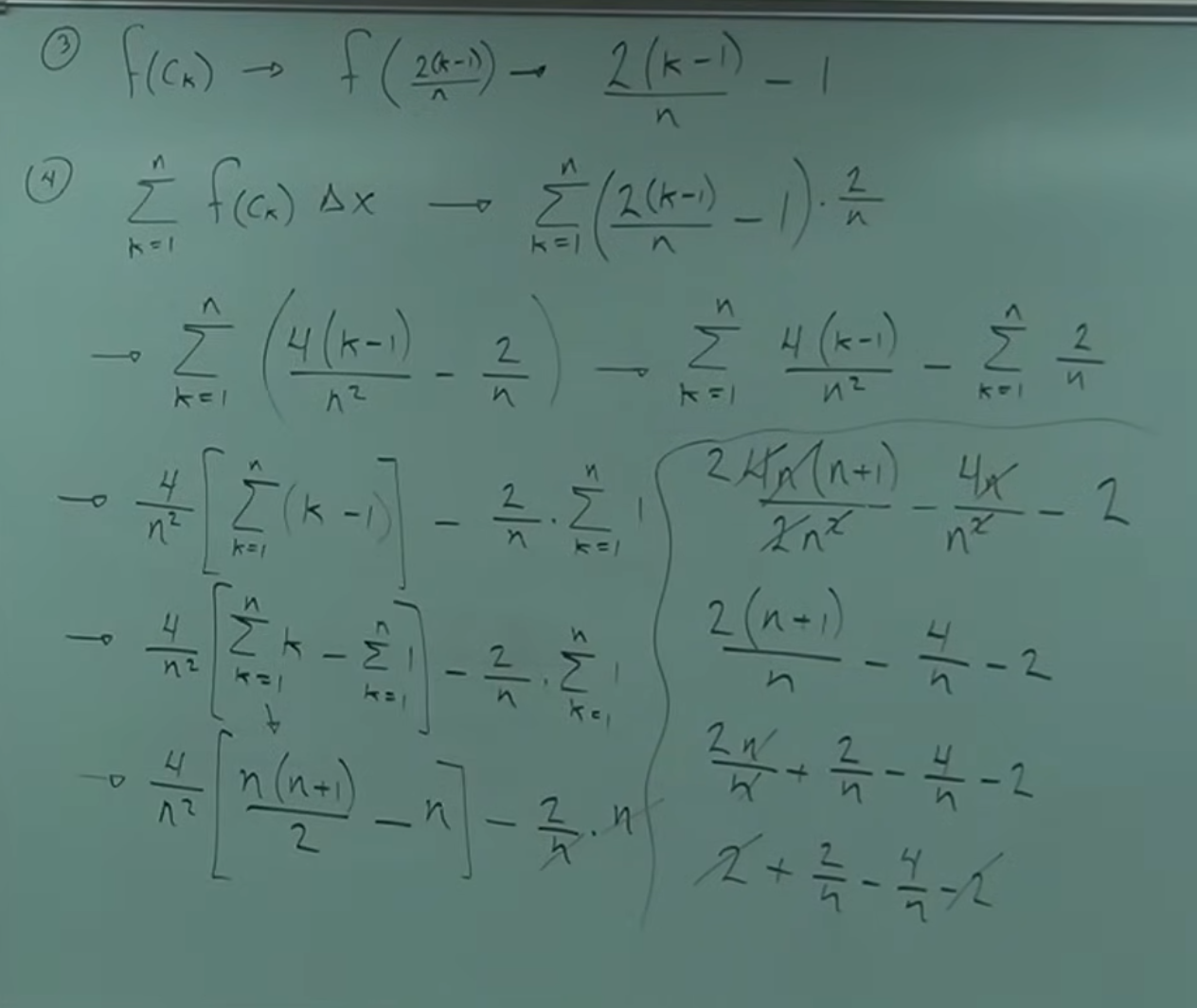
  • [1:30:30]. Step 3: Calculate $𝒇(x_{k}^{\ast})$.
    • The value $x_{k}^{\ast}$ is substituted into $𝒇(𝒙)$.
    • Substituting $x_{k}^{\ast}=\dfrac{2(k-1)}{n}$ into $𝒇(𝒙)=𝒙-1$ gives $𝒇(x_{k}^{\ast})=\dfrac{2(k-1)}{n}-1$
  • [1:32:00]. Step 4: Build the summation.
    • The approximation for the net area is $\displaystyle \sum_{k=1}^{n}\big[𝒇(x_{k}^{\ast})\cdot \Delta 𝒙\big]$
    • The values calculated earlier are substituted.
      • $\displaystyle \sum_{k=1}^{n}\left[\left(\dfrac{2(k-1)}{n}\right)-1\right]\cdot \dfrac{2}{n}$
    • Manipulating the summation.
      • $\displaystyle \sum_{k=1}^{n}\left[\dfrac{4(k-1)}{n^{2}}-\dfrac{2}{n}\right]$
      • $\displaystyle \dfrac{4}{n^{2}}\cdot \sum_{k=1}^{n}(k-1)-\dfrac{2}{n}\cdot \sum_{k=1}^{n}1$
      • $\displaystyle \dfrac{4}{n^{2}}\cdot \Big(\sum_{k=1}^{n}k-\sum_{k=1}^{n}1\Big)-\dfrac{2}{n}\cdot n$
      • $\displaystyle \dfrac{4}{n^{2}}\cdot \left(\dfrac{n(n+1)}{2}-n\right)-2$
      • $\displaystyle \dfrac{2(n+1)}{n}-\dfrac{4}{n}-2$
      • $2+\dfrac{2}{n}-\dfrac{4}{n}-2$
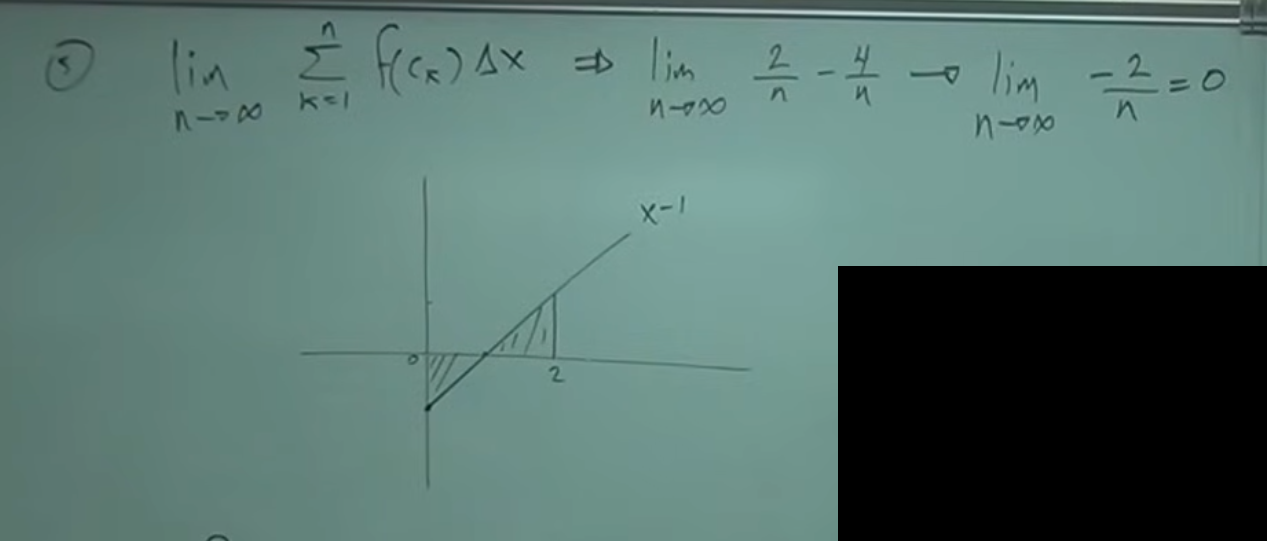
  • [1:44:30]. Step 5: Calculate the limit.
    • After evaluating the summation, the limit as $n\to\infty$ is taken.
    • The limit operation is applied to the resulting algebraic expression.
    • $\displaystyle \lim_{n\to\infty}\sum_{k=1}^{n} 𝒇(x_{k}^{\ast})\cdot \Delta 𝒙 \ \to\ \lim_{n\to\infty}\left[\dfrac{2}{n}-\dfrac{4}{n}\right]\ \to\ \lim_{n\to\infty}\left[-\dfrac{2}{n}\right]=0$
    • An area of $0$ is peculiar and suggests analyzing the graph.
  • [1:46:00]. Graphical analysis of the result.
    • The function $𝒇(𝒙)=𝒙-1$ is described as a line with slope $1$ and y-intercept $-1$.
    • The area of triangles above and below the $𝒙$-axis is computed.
    • The result is $0$ because positive and negative areas cancel each other out.
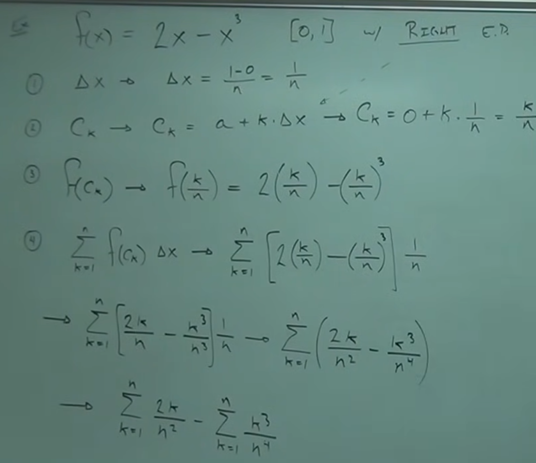
• [1:48:55]. 🧩 Example – 3: Calculating the net area under $f(x)=2x-x^{3}$ on $[0,1]$ using right endpoints. – [📷image-1] – [📷image-2]
  • Step 1: Calculate $\Delta x$
    • Formula: $\displaystyle \Delta x=\dfrac{𝓫-𝓪}{n}=\dfrac{1-0}{n}=\dfrac{1}{n}$
  • Step 2: Define the right endpoint $x_{k}^{\ast}$
    • Formula: $x_{k}^{\ast}=𝓪+k\cdot \Delta x$
    • With $𝓪=0$ and $\Delta x=\dfrac{1}{n}$ → $x_{k}^{\ast}=\dfrac{k}{n}$
  • Step 3: Evaluate the function at the right endpoint
    • $f(x_{k}^{\ast})=2\left(\dfrac{k}{n}\right)-\left(\dfrac{k}{n}\right)^{3}$
  • Step 4: Build the summation
    • Approximation: $\displaystyle \sum_{k=1}^{n} f(x_{k}^{\ast})\cdot \Delta x$
    • $\displaystyle \sum_{k=1}^{n}\left[\,\dfrac{2k}{n}-\left(\dfrac{k}{n}\right)^{3}\right]\cdot \dfrac{1}{n}$
    • $\displaystyle \sum_{k=1}^{n}\left[\dfrac{2k}{n^{2}}-\dfrac{k^{3}}{n^{4}}\right]$
    • Split: $\displaystyle \dfrac{2}{n^{2}}\sum_{k=1}^{n}k-\dfrac{1}{n^{4}}\sum_{k=1}^{n}k^{3}$
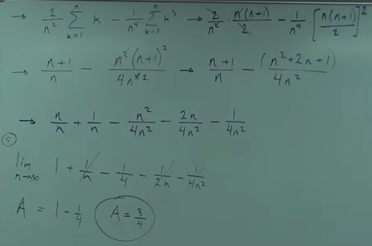
  • Step 5: Apply summation formulas
    • $\displaystyle \sum_{k=1}^{n}k=\dfrac{n(n+1)}{2}$
    • $\displaystyle \sum_{k=1}^{n}k^{3}=\left(\dfrac{n(n+1)}{2}\right)^{2}$
  • Substitution:
    • $\displaystyle \dfrac{2}{n^{2}}\cdot \dfrac{n(n+1)}{2}-\dfrac{1}{n^{4}}\cdot \left(\dfrac{n(n+1)}{2}\right)^{2} =\dfrac{n+1}{n}-\dfrac{n^{2}+2n+1}{4n^{2}} =\left(\dfrac{n}{n}+\dfrac{1}{n}\right)-\dfrac{n^{2}+2n+1}{4n^{2}}$
  • Step 6: Take the limit as $n\to\infty$
    • $\displaystyle \lim_{n\to\infty}\left[\dfrac{n+1}{n}-\dfrac{n^{2}+2n+1}{4n^{2}}\right]=\lim_{n\to\infty}\left[1+\dfrac{1}{n}-\dfrac{1}{4}-\dfrac{2}{4n}-\dfrac{1}{4n^{2}}\right] =1-\dfrac{1}{4}=\dfrac{3}{4}$
  • The net area under $f(x)=2x-x^{3}$ on $[0,1]$ is:
    • $\mathcal{A}=\dfrac{3}{4}$